Prototyping and testing

Analysis can show that a design should work. Only a test can show that it does, and only a test reveals the problems nobody thought to analyze. The Plover E2 team cannot build a full-scale aircraft in a year, but it can test the two things its design depends on most: the battery cells, whose behavior sets the mission, and the aerodynamic and handling character of the configuration, which a subscale flying model can show. Between weeks 13 and 23 the team runs both campaigns, and prepares the outline of the flight test program that a real Plover E2 would need. This lesson covers how tests are planned, run safely and interpreted, and what the team's tests found.

Testing to learn and testing to verify

Tests serve two purposes, and confusing them causes trouble. A development test is run to learn: to find out how something behaves, to calibrate a model, or to find problems early. Its plan can change as results come in, and a surprising result is a success. A verification test is run to show compliance with a requirement: its conditions, instruments, procedure and pass criteria are fixed in advance and agreed with whoever will accept the result, often the regulator, and changing them afterwards invalidates it. All of the team's tests this year are development tests. The report must say so, because a reader who sees “the subscale model stalled gently” might otherwise think the stall requirement has been verified.

Every test, of either kind, has a written plan before it starts: the objective, the article being tested and how it represents the real thing, the instruments and their accuracy, the test points in order, the pass or stop criteria for each point, the hazards and how they are controlled, and who decides to continue or stop. Sam Littlechild, who has flown flight tests for a living, reviews each plan. He tells the team that the most important line on a test card is the one that says when to stop.

Battery cell tests

Lucas sets up a test rig in the university's electrical engineering laboratory: a programmable load and power supply, a climatic chamber that can hold a cell from −30 to 60 °C, thermocouples on the cell surface and a data logger. The cells are the cylindrical type chosen for the packs, bought as samples from the supplier. The tests are of three kinds. Capacity tests discharge a fully charged cell at a constant current to its cut-off voltage at several temperatures, to measure the energy it delivers. Pulse tests apply short, high-current pulses at several states of charge and temperatures, to measure internal resistance. A small cycling test charges and discharges a few cells repeatedly with the current profile of a lesson, to begin to measure aging, though a year is far too short to reach end of life.

Cell testing is hazardous. A lithium-ion cell abused by overcharge, short circuit or overheating can vent hot flammable gas and burn. The laboratory's safety procedure requires the chamber to have a vent to the outside and an independent over-temperature cut-out, limits the number of cells in the chamber, forbids unattended overnight tests at high states of charge, and keeps a container of sand and a suitable extinguisher next to the rig. Lucas writes the test procedure so that the rig shuts down by itself if voltage, current or temperature leaves its window. The thermal runaway propagation test described in lesson 7, which deliberately drives a cell into runaway, is not run in the university laboratory; it needs a specialist test facility and is listed in the certification test program.

# Pulse test on one cell: find the internal resistance from the voltage step, at three temperatures
# (bench data recorded by the team, simplified: 10 A discharge pulse for 10 s at 50 % state of charge)
tests = {   # temperature C: list of (time s, current A, voltage V)
    20:  [(0, 0, 3.712), (1, 10, 3.403), (5, 10, 3.391), (10, 10, 3.382), (11, 0, 3.690), (40, 0, 3.708)],
    0:   [(0, 0, 3.705), (1, 10, 3.170), (5, 10, 3.148), (10, 10, 3.131), (11, 0, 3.668), (40, 0, 3.699)],
    -10: [(0, 0, 3.701), (1, 10, 2.792), (5, 10, 2.757), (10, 10, 2.731), (11, 0, 3.633), (40, 0, 3.694)],
}
datasheet_20C = 0.030
for T, d in tests.items():
    v0, i_p = d[0][2], d[1][1]
    r_inst = (v0 - d[1][2]) / i_p             # ohmic part: step within 1 s
    r_10s = (v0 - d[3][2]) / i_p              # includes the slower polarization
    print(f'{T:4d} C: R(1 s) {r_inst*1000:5.1f} mOhm   R(10 s) {r_10s*1000:5.1f} mOhm   ratio to 20 C {r_10s/((tests[20][0][2]-tests[20][3][2])/10):4.2f}')
r20 = (tests[20][0][2] - tests[20][3][2]) / 10
print(f'\nmeasured 10 s resistance at 20 C: {r20*1000:.1f} mOhm against {datasheet_20C*1000:.0f} mOhm on the data sheet ({(r20/datasheet_20C-1)*100:+.0f} %)')
# what the measured values mean for the pack: 108 series groups of 30 cells
for T, d in tests.items():
    r = (d[0][2] - d[3][2]) / 10
    R_pack = r / 30 * 108
    I = 65_400 / 394                          # take-off and climb current at nominal voltage
    print(f'{T:4d} C: pack resistance {R_pack*1000:5.1f} mOhm, voltage drop at take-off {I*R_pack:5.1f} V, heat {I**2*R_pack/1000:4.1f} kW')

  20 C: R(1 s)  30.9 mOhm   R(10 s)  33.0 mOhm   ratio to 20 C 1.00
   0 C: R(1 s)  53.5 mOhm   R(10 s)  57.4 mOhm   ratio to 20 C 1.74
 -10 C: R(1 s)  90.9 mOhm   R(10 s)  97.0 mOhm   ratio to 20 C 2.94

measured 10 s resistance at 20 C: 33.0 mOhm against 30 mOhm on the data sheet (+10 %)
  20 C: pack resistance 118.8 mOhm, voltage drop at take-off  19.7 V, heat  3.3 kW
   0 C: pack resistance 206.6 mOhm, voltage drop at take-off  34.3 V, heat  5.7 kW
 -10 C: pack resistance 349.2 mOhm, voltage drop at take-off  58.0 V, heat  9.6 kW

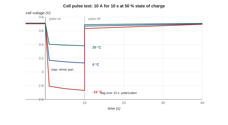
The pulse tests give two numbers at each temperature. The instantaneous voltage step, within a second of the pulse starting, measures the purely ohmic resistance of the cell's electrodes, electrolyte and connections. The further sag over the next ten seconds adds the slower polarization of the electrochemical reactions. For the power demands of a flight, which last minutes, the 10-second value is the better one to use. At 20 °C it is 33.0 milliohms, 10 percent above the data sheet's 30. At −10 °C it is 97 milliohms, 2.94 times the 20 °C value; the simulation in lesson 6 had assumed a factor of 2.2.

Both differences go the wrong way, and the team reruns the mission simulation with the measured values. At end of life and 20 °C the mission still passes, with 6.9 percent remaining instead of 7.4 and a lowest cell voltage of 3.01 V. But the pack pre-warmed to 15 °C, which passed before, now fails narrowly: its lowest voltage falls to 2.98 V. The team raises the take-off limit in the draft flight manual from 15 to 20 °C of pack temperature, and asks the charger supplier whether the pre-conditioning heater can reach 20 °C in an unheated hangar in winter. This is exactly what development tests are for: a 10 percent difference found on the bench in week 15 is a change to a limit; found in certification flight testing, it would be a change to the battery.

The subscale demonstrator

The second campaign is a quarter-scale flying model of the Plover E2. A subscale model cannot show everything, and choosing what it should show decides how it is built. The team wants it to show the stall behavior, the static and dynamic stability in pitch, and the handling with the center of gravity at the forward and aft limits. Those are dynamic questions, which depend on the model's mass, inertia and speed as well as its shape, so the model must be dynamically scaled. For motion under gravity, the right similarity is Froude scaling, which keeps the ratio of inertial to gravitational forces the same: lengths scale with \(\lambda\), speeds with \(\sqrt{\lambda}\), masses with \(\lambda^{3}\), moments of inertia with \(\lambda^{5}\) and times with \(\sqrt{\lambda}\).

# Subscale demonstrator for the Plover E2: Froude scaling and the flight test point matrix
import math
lam = 0.25                                       # geometric scale (quarter scale)
full = {'span m': 12.4, 'mass kg': 770.0, 'speed m/s': 46.3, 'Iyy kg m2': 1050.0, 'time s': 1.0}
print(f'quarter-scale demonstrator, dynamically scaled (Froude):')
print(f'  span {full["span m"]*lam:.2f} m')
print(f'  mass {full["mass kg"]*lam**3:.1f} kg (lambda^3)')
print(f'  speed {full["speed m/s"]*math.sqrt(lam):.1f} m/s (sqrt lambda)')
print(f'  pitch inertia {full["Iyy kg m2"]*lam**5:.3f} kg m2 (lambda^5)')
print(f'  time {math.sqrt(lam):.2f} s per full-scale second: a 3 s short-period cycle lasts {3*math.sqrt(lam):.1f} s')
nu = 1.5e-5
Re_full = 46.3 * 1.13 / nu
Re_sub = 46.3 * math.sqrt(lam) * 1.13 * lam / nu
print(f'  Reynolds number {Re_sub:.2e} against {Re_full:.2e} full scale (ratio {Re_sub/Re_full:.3f})')
print(f'  limit for small drones in the sponsor operations manual: 25 kg; scaled mass ok: {full["mass kg"]*lam**3 <= 25}')

# build-up test matrix: each block must be flown and reviewed before the next
blocks = [('taxi and hops', ['fwd'], [0.6, 0.8], ['flap 0']),
          ('handling and trim', ['fwd', 'mid', 'aft'], [1.3, 1.6, 2.0], ['flap 0', 'flap full']),
          ('stalls', ['fwd', 'aft'], [1.0], ['flap 0', 'flap full']),
          ('stability tests (doublets)', ['fwd', 'mid', 'aft'], [1.3, 1.6, 2.0], ['flap 0']),
          ('motor cut and glide', ['mid'], [1.3, 1.6], ['flap 0'])]
total, per_flight = 0, 6
for name, cgs, speeds, flaps in blocks:
    pts = len(cgs) * len(speeds) * len(flaps)
    total += pts
    print(f'{name:28s} {len(cgs)} CG x {len(speeds)} speeds x {len(flaps)} flap = {pts:2d} points, {math.ceil(pts/per_flight)} flight{"s" if math.ceil(pts/per_flight) > 1 else ""}')
print(f'total {total} test points, at least {math.ceil(total/per_flight)} flights of {per_flight} points (speeds as multiples of the stall speed)')

quarter-scale demonstrator, dynamically scaled (Froude):
  span 3.10 m
  mass 12.0 kg (lambda^3)
  speed 23.1 m/s (sqrt lambda)
  pitch inertia 1.025 kg m2 (lambda^5)
  time 0.50 s per full-scale second: a 3 s short-period cycle lasts 1.5 s
  Reynolds number 4.36e+05 against 3.49e+06 full scale (ratio 0.125)
  limit for small drones in the sponsor operations manual: 25 kg; scaled mass ok: True
taxi and hops                1 CG x 2 speeds x 1 flap =  2 points, 1 flight
handling and trim            3 CG x 3 speeds x 2 flap = 18 points, 3 flights
stalls                       2 CG x 1 speeds x 2 flap =  4 points, 1 flight
stability tests (doublets)   3 CG x 3 speeds x 1 flap =  9 points, 2 flights
motor cut and glide          1 CG x 2 speeds x 1 flap =  2 points, 1 flight
total 35 test points, at least 6 flights of 6 points (speeds as multiples of the stall speed)

At quarter scale the model has a span of 3.10 m, a mass of 12.0 kg and a flying speed of 23 m/s for the full-scale cruise, and everything happens twice as fast: a 3-second short-period oscillation of the real aircraft takes 1.5 seconds on the model. Getting the mass and inertia right is harder than getting the shape right. The model is built from a commercial kit airframe of nearly the right planform, modified with a new tail and wing tips, and ballast is placed so that the mass, center of gravity and pitch inertia match the scaled values. Hélène helps the team swing the model on a bifilar pendulum to measure its inertia, adding and moving ballast until the period matches.

What the model cannot match is the Reynolds number, which is one-eighth of the full-scale value. At the model's Reynolds number of about 440,000, boundary layers behave differently: laminar separation bubbles form more easily, maximum lift is lower and the stall can be more abrupt. The team therefore treats the model's stall speed as unrepresentative and looks only at the character of the stall: whether the wing drops, whether the stall starts at the root as designed, and whether recovery is prompt. Tufts on the wing, filmed by a small camera on the fin, show where the flow separates first.

The model is flown as a remotely piloted aircraft under a remote pilot certificate under 14 CFR Part 107, at a model aircraft field east of Wichita, with a pilot who holds the certificate and a safety officer who can terminate the flight. It carries a small autopilot that records attitude, rates, accelerations, airspeed and control positions at 50 samples per second, and a flight termination function that cuts the motor and deploys full up elevator and rudder, a configuration that puts the model into a slow, stable descent. Lucas arranged the flying site approval in week 8, as the risk register required.

The test points follow a build-up: start with the least demanding conditions and expand only when the data from the previous block have been reviewed and understood. The matrix gives 35 test points in about eight flights. In practice the team flies eleven, because two flights are lost to wind above the limit and one to a data logger that did not start, a ratio Sam says is typical of real flight testing.

What the model showed

Three findings matter for the design. The stall begins at the wing root and spreads outward, as intended by the aerofoil choice and a slight washout, and the model does not drop a wing with the center of gravity at the forward or mid positions. At the aft limit, the model shows a mild tendency to drop the right wing at the stall, which the team traces to the propeller slipstream over the left wing root. The fix, a small stall strip on the right wing's leading edge near the root, is a classic one on light aircraft, and a second flight with the strip shows a straight stall.

The pitch doublets, quick forward-and-back stick inputs, excite the short-period mode. Fitting a damped oscillation to the recorded pitch rate gives a period of 1.6 seconds and a damping ratio of 0.55 on the model, which scale to a full-scale period of 3.2 seconds, close to the 3 seconds estimated in lesson 6. The phugoid could not be measured: in a few hundred meters of airspace the model never flew long enough without a correction. Motor cut and glide tests show a glide ratio of about 11, well below the full-scale estimate of 15, as expected at the low Reynolds number.

The team is careful in the report about what these results mean. They are evidence that the configuration has no gross stability or stall problems, and that the stall strip is needed. They are not measurements of the full-scale aircraft's stall speed, glide ratio or handling qualities.

The full-scale flight test program

For the certification plan, Grace and Sam outline the flight test program a real Plover E2 would need. It would start with ground tests of the electric drive on an iron bird, a ground rig with the real motor, inverter, battery and cooling system, run through hundreds of hours of simulated lessons before the first flight. The first aircraft would then fly an envelope expansion: low-speed taxi, high-speed taxi, first flight in the circuit, then step by step to the edges of the speed, load factor and center of gravity envelope. Flutter tests would clear the speed envelope in small steps with excitation and monitoring. Spin tests, required for the utility category approval, would fly with an emergency spin recovery parachute on the tail, at a safe altitude, starting with incipient spins. Battery tests would include charging and flight at the temperature limits.

Kenji estimates the full program at about 450 flight hours over 18 months with two test aircraft. That number goes into the cost and schedule estimate in lesson 10.