Experimental research: apparatus, calibration and the lab notebook

An experiment is only as good as its weakest measurement. In a teaching laboratory, the apparatus has been tested by generations of students and the dominant sources of error are known. In a research project, you build or assemble the apparatus yourself, you discover its weaknesses by using it, and you must establish, by calibration, that each instrument measures what you think it measures. This lesson follows Maya from an empty bench to a working experiment: designing the apparatus around the measurements the hypotheses require, calibrating the instruments against known references, finding and fixing a systematic error, and keeping a laboratory notebook good enough that someone else could repeat the work from it.

Designing the apparatus

Lesson 5 turned Maya's question into required measurements: the transit time of the magnet through each pipe to about 1 per 100, the magnet's dipole moment to 1 or 2 per 100, each pipe's conductivity to about 1 per 100, and each pipe's inner and outer radius to a few hundredths of a millimetre. Her apparatus followed directly from that list. A vertical aluminium frame held each pipe plumb, checked with a spirit level and a plumb line. Two infrared light gates, mounted on short slotted sections of plastic tube attached above and below the copper, were replaced by a better arrangement after a week: small slots cut through the pipe wall at 0.100 m and 0.900 m from the top, just wide enough for a light beam, with the gates clamped outside. The slots were short enough not to disturb the eddy currents measurably, a claim she later tested by comparing transit times with and without tape over the slots. A microcontroller recorded the gate transitions with a resolution of 0.1 ms.

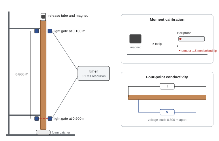
The magnet was released from rest inside a short plastic guide tube that centred it on the pipe axis. Because the magnet reaches terminal speed within a few millimetres, as lesson 1's estimate showed, the gate 0.100 m below the top was far enough to be sure the speed was constant over the timed section. That assumption is itself testable: with a third gate at 0.500 m, the two halves of the baseline should give the same speed, and in Maya's tests they agreed to within 0.3 per 100. Small checks like this are cheap to build in and make the thesis much more convincing, because they turn assumptions into measurements.

Calibrating the dipole moment

The dipole moment of a permanent magnet is not printed on the package. A grade such as N42 specifies a range of remanent magnetization, which for Maya's magnet implied a moment between about 1.55 and 1.70 A m², a spread of 9 per 100. Since the predicted drag is proportional to the square of the moment, that spread alone would make an 18 per 100 uncertainty in the prediction, far too large. She therefore measured the moment. On the axis of a point dipole the field at distance \(z\) is \(B = \mu_0 m/(2\pi z^3)\), so measuring \(B\) at several distances with a Hall probe gives \(m\). For a finite cylinder of radius \(R\) and length \(L\), uniformly magnetized, the exact field on the axis is

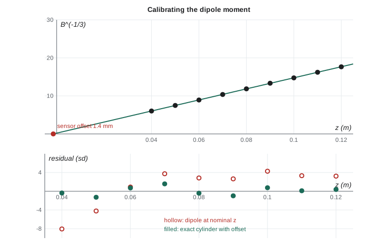
which approaches the dipole form when \(z\) is much larger than \(R\) and \(L\). At 40 mm the two differ by about 1 per 100, and at 100 mm by about 0.2 per 100. Maya first fitted the simple dipole formula to readings from 40 to 120 mm, measured from the centre of the magnet to the tip of the probe, and obtained a moment of about 1.50 A m². That was below the manufacturer's range, which was the first sign of trouble. Worse, the fit residuals were not random: the dipole model was systematically too steep, as though the distances were all slightly too small.

Finding a systematic error

A systematic error is one that shifts every measurement in the same direction, so repetition does not reduce it. Unlike random errors, systematic errors are invisible in the scatter of repeated readings; they show up only when the data are compared with something independent, such as a model, a second method or a known standard. Maya's residuals were the clue. If every distance were too small by the same amount \(z_0\), the true distance would be \(z + z_0\), and the dipole formula could be rearranged into a straight line:

so a plot of \(B^{-1/3}\) against the nominal distance \(z\) should be a straight line whose slope gives \(m\) and whose intercept gives the offset \(z_0\). Her fit gave an offset of about 1.4 mm. The Hall probe's data sheet, which she then read more carefully, explained it: the sensing element sits 1.5 mm behind the tip of the protective housing. Every distance she had recorded was 1.5 mm too short; the linearized fit's slightly smaller value comes from the near-field departure from the dipole form, which the straight-line model ignores. It is the kind of error that is obvious in hindsight and nearly invisible in advance, and it is common enough that experienced experimentalists check the location of the active element in every probe they use. Correcting the offset to the data-sheet value and fitting the exact cylinder formula gave a moment of about 1.62 A m², inside the manufacturer's range, with residuals that scattered randomly.

import math, random
MU0 = 4e-7*math.pi
R, L = 6.35e-3, 12.70e-3
def b_exact(m, z):
    M = m/(math.pi*R*R*L)
    return MU0*M/2*((z + L/2)/math.hypot(z + L/2, R) - (z - L/2)/math.hypot(z - L/2, R))
# synthetic readings: true moment 1.62 A m^2, sensor 1.5 mm behind the tip, probe noise
rnd = random.Random(606)
z_nom = [0.040 + 0.010*i for i in range(9)]                       # 40 to 120 mm
B = [b_exact(1.62, z + 0.0015)*(1 + rnd.gauss(0, 0.004)) + rnd.gauss(0, 2e-6) for z in z_nom]
sB = [math.hypot(0.004*b, 2e-6) for b in B]
def wls(x, y, s):                                     # weighted straight-line fit y = p + q x
    w = [1/si**2 for si in s]
    S, Sx, Sy = sum(w), sum(wi*xi for wi, xi in zip(w, x)), sum(wi*yi for wi, yi in zip(w, y))
    Sxx, Sxy = sum(wi*xi*xi for wi, xi in zip(w, x)), sum(wi*xi*yi for wi, xi, yi in zip(w, x, y))
    D = S*Sxx - Sx*Sx
    p, q = (Sxx*Sy - Sx*Sxy)/D, (S*Sxy - Sx*Sy)/D
    return p, q, math.sqrt(Sxx/D), math.sqrt(S/D)
# fit 1: dipole, nominal distances, B = (MU0 m / 2 pi) * z^-3 through the origin
x = [z**-3 for z in z_nom]
w = [1/s**2 for s in sB]
c = sum(wi*xi*bi for wi, xi, bi in zip(w, x, B))/sum(wi*xi*xi for wi, xi in zip(w, x))
m1 = 2*math.pi*c/MU0
res1 = [(b - c*xi)/s for b, xi, s in zip(B, x, sB)]
print(f"fit 1, dipole at nominal z: m = {m1:.3f} A m^2, residuals {[round(r, 1) for r in res1]}")
# fit 2: linearized dipole, B^(-1/3) = k (z + z0)
y = [b**(-1/3) for b in B]; sy = [s*b**(-4/3)/3 for b, s in zip(B, sB)]
p, q, sp, sq = wls(z_nom, y, sy)
z0 = p/q
m2 = 2*math.pi/(MU0*q**3)
print(f"fit 2, linearized: offset z0 = {z0*1e3:.2f} mm, m = {m2:.3f} A m^2")
# fit 3: exact cylinder formula with the offset, linear in m
z0 = 0.0015                                         # data-sheet offset, confirmed by fit 2
f = [b_exact(1.0, z + z0) for z in z_nom]
m3 = sum(wi*fi*bi for wi, fi, bi in zip(w, f, B))/sum(wi*fi*fi for wi, fi in zip(w, f))
sm3 = 1/math.sqrt(sum(wi*fi*fi for wi, fi in zip(w, f)))
res3 = [(b - m3*fi)/s for b, fi, s in zip(B, f, sB)]
chi2 = sum(r*r for r in res3)
print(f"fit 3, exact cylinder with offset: m = {m3:.3f} +/- {sm3:.3f} A m^2 (statistical)")
print(f"       residuals {[round(r, 1) for r in res3]}, chi-squared {chi2:.1f} for {len(B) - 1} degrees of freedom")
print(f"remanent field implied: {MU0*m3/(math.pi*R*R*L):.3f} T")

fit 1, dipole at nominal z: m = 1.513 A m^2, residuals [-8.1, -4.2, 0.9, 3.7, 2.8, 2.6, 4.3, 3.3, 3.2]
fit 2, linearized: offset z0 = 1.41 mm, m = 1.623 A m^2
fit 3, exact cylinder with offset: m = 1.622 +/- 0.003 A m^2 (statistical)
       residuals [-0.4, -1.3, 0.7, 1.6, -0.4, -1.0, 0.8, 0.1, 0.4], chi-squared 6.6 for 8 degrees of freedom
remanent field implied: 1.267 T

The output tells the story. The naive fit gives a moment about 7 per 100 too low, with residuals that run from negative to positive across the range, the signature of a model missing something. The linearized fit recovers an offset of about 1.4 mm, close to the data-sheet value. The exact fit with the offset gives a moment of 1.62 A m² with a statistical uncertainty of about 0.2 per 100 and a chi-squared close to the number of degrees of freedom, which says the remaining scatter is consistent with the stated probe noise. The statistical uncertainty is not the whole story, however. The Hall probe's gain was itself calibrated against the field at the centre of a Helmholtz coil, computed from its dimensions and current, to about 0.5 per 100, and the rail positions were known to 0.1 mm. Combining these, Maya quoted \(m = 1.62 \pm 0.02\) A m², an uncertainty of about 1 per 100 dominated by the probe gain and position.

Calibrating the conductivity

Handbook values for the conductivity of copper refer to pure annealed copper, about \(5.8 \times 10^{7}\) S/m at 20 degrees. Copper water pipe is usually a phosphorus-deoxidized alloy whose conductivity is about 85 per 100 of that standard, and the exact value varies with composition and temper. Maya measured each pipe with a four-point method: a steady current \(I\) through the whole pipe from end clamps, and the voltage \(V\) measured by two separate leads clipped a distance \(\ell\) apart. Because almost no current flows in the voltage leads, contact resistances do not affect the reading, which is the reason for using four points rather than two. With the wall cross-section \(A = \pi(b^2 - a^2)\) from micrometer measurements, the conductivity is \(\sigma = I \ell/(V A)\). The voltages are small, about 2 millivolts at 5 A for her copper pipes, so she used a nanovoltmeter, reversed the current to cancel thermoelectric offsets, and recorded the pipe temperature, since copper's resistance changes by about 0.4 per 100 per degree.

import math
I, ell = 5.000, 0.800                          # current (A), voltage-lead spacing (m)
OD = [15.874, 15.878, 15.877, 15.873]          # micrometer, mm, four positions
wall = [1.019, 1.023, 1.018, 1.021]            # mm
Vfwd, Vrev = [1.7071e-3, 1.7083e-3, 1.7078e-3], [-1.7039e-3, -1.7044e-3, -1.7046e-3]
T = 21.4                                       # pipe temperature, degrees
mean = lambda v: sum(v)/len(v)
def sem(v):
    m = mean(v); return math.sqrt(sum((x - m)**2 for x in v)/(len(v) - 1)/len(v))
b = mean(OD)/2*1e-3; w = mean(wall)*1e-3; a = b - w
A = math.pi*(b*b - a*a)
V = (mean(Vfwd) - mean(Vrev))/2                # current reversal removes thermal offsets
offset = (mean(Vfwd) + mean(Vrev))/2
sigma = I*ell/(V*A)
sigma20 = sigma*(1 + 0.00393*(T - 20))         # refer to 20 degrees
print(f"inner radius a = {a*1e3:.3f} mm, wall w = {w*1e3:.3f} mm, area A = {A*1e6:.3f} mm^2")
print(f"thermal offset removed: {offset*1e6:.2f} microvolts")
print(f"sigma at {T} degrees = {sigma:.3e} S/m;  at 20 degrees = {sigma20:.3e} S/m")
print(f"as a fraction of the annealed copper standard (5.80e7): {sigma20/5.80e7:.3f}")

inner radius a = 6.918 mm, wall w = 1.020 mm, area A = 47.614 mm^2
thermal offset removed: 1.72 microvolts
sigma at 21.4 degrees = 4.924e+07 S/m;  at 20 degrees = 4.951e+07 S/m
as a fraction of the annealed copper standard (5.80e7): 0.854

The result, about \(4.9 \times 10^{7}\) S/m or 85 per 100 of the annealed standard, matched the expected value for phosphorus-deoxidized pipe and was used for all three half-inch copper pipes after spot checks showed they agreed within 1 per 100. The largest contribution to the uncertainty came not from the voltmeter but from the wall thickness, which varied by a few micrometres around the circumference and along the length. That finding shaped the uncertainty budget in lesson 8: for the conductivity, as for the drag, the dimensions of the pipe matter more than the electronics.

The laboratory notebook

A laboratory notebook is the primary record of an experiment. It should allow you, months later, and anyone else, to reconstruct what was done, when, with what equipment and settings, and what was observed, including what went wrong. Paper notebooks with numbered pages remain common; electronic notebooks are increasingly standard in research groups and have the advantage of search and links to data files. Either way, the rules are similar. Date every entry. Write as you work, not afterward. Record raw readings and settings, not just processed results. Record equipment serial numbers and software versions. Never erase or delete: cross out errors with a single line so they remain readable, and note why. Sketch the setup. Record ideas and hunches as well as data, because the reason you tried something is often as useful later as the result.

Maya's notebook entry for the day she found the probe offset reads, in part: "Calibration run 3: dipole fit gives m = 1.50, below the manufacturer's range. Residuals systematic, model too steep. Hypothesis: distance offset. Linearized fit gives z0 = 1.4 mm. Data sheet section 4: active element 1.5 mm behind tip. All distances in runs 1 to 3 short by 1.5 mm. Rerun with corrected rail zero tomorrow." Six lines written in ten minutes saved her a day of reconstruction when she wrote the methods chapter, and gave her examiners a clear account of how the error was found. A good notebook is also an integrity record: it shows that data were not selected or adjusted after the fact, which lesson 9 explains matters more than students often realize.

Testing the apparatus with controls

Before collecting the main data, Maya ran the two controls planned in lesson 5. The slotted copper pipe, in which eddy currents cannot circulate around the circumference, gave a transit time between the gates of 0.287 seconds, within 1 per 100 of the 0.286 seconds expected for free fall from rest at the top, which validated the timing system. The nonmagnetic steel slug, dropped through each copper pipe, also fell freely within the timing uncertainty, showing that wall friction from a magnet-sized object was negligible when the object was not magnetically attracted to anything. These controls do not test the eddy-current physics; they test that nothing else is happening. A result that survives the controls can be attributed to the physics with much more confidence.