Electrons in a periodic potential: Bloch's theorem and nearly-free electrons

The free-electron model of lesson 7 ignores the ions altogether, yet it explains a great deal. It cannot, however, explain why some solids are insulators, why aluminium's Hall coefficient can be positive, or why electrons in a perfect crystal do not scatter from the ions they pass. All three puzzles are resolved by taking the periodic potential of the lattice seriously. This lesson proves Bloch's theorem, which says what electron wave functions in any periodic potential must look like, and then treats a weak periodic potential as a perturbation. The result is the most important idea in the physics of solids: the energies available to an electron form bands, separated by gaps in which no states exist.

Bloch's theorem

An electron in a crystal moves in a potential \(U(\mathbf r)\) that has the periodicity of the lattice, \(U(\mathbf r + \mathbf R) = U(\mathbf r)\) for every lattice vector \(\mathbf R\). This potential includes the attraction of the ions and the average repulsion of all the other electrons, in the independent-electron approximation that treats each electron as moving in an average field. The Schrödinger equation is \(H\psi = [-\hbar^2\nabla^2/2m + U(\mathbf r)]\psi = E\psi\).

Define the translation operator \(T_{\mathbf R}\), which shifts a function by \(\mathbf R\): \(T_{\mathbf R}\psi(\mathbf r) = \psi(\mathbf r + \mathbf R)\). Because the kinetic energy is unchanged by translation and the potential is periodic, \(T_{\mathbf R}\) commutes with \(H\). Translations also commute with each other: \(T_{\mathbf R}T_{\mathbf R'} = T_{\mathbf R + \mathbf R'}\). A set of commuting operators can be diagonalized simultaneously, as PHYS-372 established, so we can choose energy eigenstates that are also eigenstates of every \(T_{\mathbf R}\), with eigenvalues \(c(\mathbf R)\). The composition rule requires \(c(\mathbf R + \mathbf R') = c(\mathbf R)c(\mathbf R')\), and normalization over a large crystal with periodic boundary conditions requires \(|c| = 1\). The only functions with these properties are exponentials, \(c(\mathbf R) = e^{i\mathbf k\cdot\mathbf R}\), for some vector \(\mathbf k\). Therefore

This is Bloch's theorem, proved by Felix Bloch in his 1928 doctoral thesis under Heisenberg (the one-dimensional mathematics had been worked out by Gaston Floquet in 1883 for differential equations with periodic coefficients). An equivalent statement is that every eigenstate can be written as

a plane wave modulated by a function with the periodicity of the lattice. To verify, \(\psi(\mathbf r + \mathbf R) = e^{i\mathbf k\cdot(\mathbf r + \mathbf R)}u(\mathbf r + \mathbf R) = e^{i\mathbf k\cdot\mathbf R}\psi(\mathbf r)\). The label \(n\), the band index, distinguishes the different solutions with the same \(\mathbf k\).

What Bloch's theorem implies

Several consequences follow immediately. First, \(\mathbf k\) is defined only up to a reciprocal lattice vector, because \(e^{i(\mathbf k + \mathbf G)\cdot\mathbf R} = e^{i\mathbf k\cdot\mathbf R}\). So, as for phonons in lesson 5, every state can be labelled by a wave vector in the first Brillouin zone. With periodic boundary conditions on a crystal of \(N\) cells, there are exactly \(N\) allowed \(\mathbf k\) values in the zone, so each band holds \(N\) orbital states, or \(2N\) electrons counting spin. This counting decides in lesson 9 which materials are metals.

Second, \(\hbar\mathbf k\) is not the momentum of the electron. A Bloch state is not an eigenstate of the momentum operator, because \(u_{n\mathbf k}\) contains many Fourier components. \(\hbar\mathbf k\) is the crystal momentum, conserved in collisions only up to \(\hbar\mathbf G\), exactly as for phonons.

Third, and most remarkable, a Bloch state extends through the whole crystal with constant probability density in each cell, \(|\psi(\mathbf r + \mathbf R)|^2 = |\psi(\mathbf r)|^2\). An electron in such a state travels through the perfect lattice without scattering at all. Its average velocity, shown in more advanced treatments, is \(\mathbf v = \hbar^{-1}\nabla_{\mathbf k}E_n(\mathbf k)\), the group velocity of the wave packet, and it stays constant in the absence of external forces. This is why Sommerfeld's mean free paths in lesson 7 can be hundreds of atomic spacings. Electrons are scattered only by deviations from periodicity: thermal vibrations, impurities, vacancies and boundaries.

Fourth, for each band, \(E_n(\mathbf k)\) is a continuous, periodic function of \(\mathbf k\) in reciprocal space. The set of these functions is the band structure of the crystal, and computing and measuring it is the central task of electronic structure physics.

Nearly free electrons

To see how gaps arise, consider a weak periodic potential. Expand it in the reciprocal lattice of lesson 3, \(U(\mathbf r) = \sum_{\mathbf G}U_{\mathbf G}e^{i\mathbf G\cdot\mathbf r}\), with \(U_{-\mathbf G} = U_{\mathbf G}^*\) because \(U\) is real, and choose the zero of energy so that \(U_0 = 0\). Without the potential, the eigenstates are plane waves \(e^{i\mathbf k\cdot\mathbf r}\) with energy \(\varepsilon_{\mathbf k} = \hbar^2k^2/2m\). The potential couples a plane wave \(\mathbf k\) only to plane waves \(\mathbf k - \mathbf G\), with matrix element \(U_{\mathbf G}\).

For most \(\mathbf k\), the coupled states differ greatly in energy, and second-order perturbation theory from PHYS-373 gives only a small shift of order \(|U_{\mathbf G}|^2/(\varepsilon_{\mathbf k} - \varepsilon_{\mathbf k - \mathbf G})\). But when \(\varepsilon_{\mathbf k} = \varepsilon_{\mathbf k - \mathbf G}\), the two states are degenerate and must be treated together with degenerate perturbation theory. The condition \(|\mathbf k| = |\mathbf k - \mathbf G|\) is exactly the condition for \(\mathbf k\) to lie on a Brillouin zone boundary, the Bragg plane of \(\mathbf G\). Keeping just these two plane waves, \(\psi = \alpha e^{i\mathbf k\cdot\mathbf r} + \beta e^{i(\mathbf k - \mathbf G)\cdot\mathbf r}\), the Schrödinger equation becomes

Exactly on the zone boundary, where \(\varepsilon_{\mathbf k} = \varepsilon_{\mathbf k - \mathbf G}\), the two energies are \(\varepsilon_{\mathbf k} \pm |U_{\mathbf G}|\): a gap of

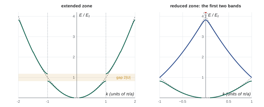
opens in the spectrum. Away from the boundary, the bands approach the free-electron parabola. Near the boundary, they bend away from it and meet the boundary with zero slope, so the group velocity of an electron at the zone boundary vanishes: like the phonon at the edge of the zone, it is a standing wave.

The physical reason is Bragg reflection. An electron wave with \(\mathbf k\) on the zone boundary satisfies the Bragg condition, so the lattice reflects it into \(\mathbf k - \mathbf G\), and the two combine into standing waves. In one dimension, with \(k = \pi/a\), the two standing waves are \(\cos(\pi x/a)\) and \(\sin(\pi x/a)\). The first piles electron density onto the ions, where the potential is most negative, and has lower energy; the second puts its density between the ions and has higher energy. The difference between their potential energies is the gap.

Extended, reduced and repeated zones

Bands can be drawn in three equivalent ways. In the extended zone scheme, each band is drawn in its own Brillouin zone, so the picture resembles the free-electron parabola with breaks at the zone boundaries. In the reduced zone scheme, every band is translated by reciprocal lattice vectors into the first zone, so each \(\mathbf k\) in the zone carries a stack of energies \(E_1(\mathbf k), E_2(\mathbf k), \dots\). In the repeated zone scheme, each band is drawn periodically throughout \(\mathbf k\)-space. The reduced zone scheme is the most common, and it is how computed and measured band structures are almost always displayed.

An exactly solvable model: Kronig–Penney

In 1931, Ralph Kronig and William Penney solved a one-dimensional crystal of square potential barriers exactly. In the limit of very narrow, high barriers spaced by \(a\), the condition for an allowed energy reduces to

where \(P\) measures the strength of the barriers. Since \(|\cos ka| \le 1\), energies for which the right side exceeds 1 in magnitude are forbidden. The program scans the energy, finds the allowed bands for a strong barrier, \(P = 3\pi/2\), and then compares the first gap for weak barriers with the nearly-free-electron prediction.

import math
# Kronig-Penney model: electrons in a periodic array of square barriers.
# Allowed energies satisfy |f(E)| <= 1, f = cos(alpha a) + P sin(alpha a)/(alpha a) in the delta-barrier limit.
P = 3 * math.pi / 2          # barrier strength m V0 b a / hbar^2
def f(x):                     # x = alpha a = sqrt(2 m E) a / hbar
    return math.cos(x) + P * math.sin(x) / x
# scan x = alpha a and record band edges, then express energy in units of E1 = hbar^2 pi^2 / (2 m a^2)
xs = [1e-6 + i * 4 * math.pi / 200000 for i in range(200001)]
edges, inside = [], False
for x in xs:
    ok = abs(f(x)) <= 1
    if ok != inside:
        edges.append(x); inside = ok
if inside: edges.append(xs[-1])
print(f"Kronig-Penney, P = 3 pi/2; energies in units of the infinite-well ground state E1")
for i in range(0, len(edges) - 1, 2):
    lo, hi = (edges[i] / math.pi) ** 2, (edges[i + 1] / math.pi) ** 2
    print(f"  band {i // 2 + 1}: E from {lo:6.3f} to {hi:6.3f} E1   (width {hi - lo:.3f})")
    if i + 2 < len(edges):
        print(f"           gap of {(edges[i + 2] / math.pi) ** 2 - hi:.3f} E1")
print()
# Weak potential: compare the numerical first gap with the nearly-free-electron prediction 2|U_G|
for P in (0.05, 0.2, 0.5):
    g = lambda x: math.cos(x) + P * math.sin(x) / x
    # the first gap opens just above x = pi, where g passes below -1
    lo = math.pi
    a, b = math.pi * 1.0000001, math.pi * 1.5
    for _ in range(80):
        m = (a + b) / 2
        if g(m) < -1: a = m
        else: b = m
    gap = (b / math.pi) ** 2 - 1
    # for delta barriers, U_G = U_0 is the same for every G: 2|U_G| = 2 * (2 P / pi^2) E1
    print(f"  P = {P:4.2f}: first gap {gap:.4f} E1, nearly-free-electron estimate 4P/pi^2 = {4 * P / math.pi ** 2:.4f} E1")

Kronig-Penney, P = 3 pi/2; energies in units of the infinite-well ground state E1
  band 1: E from  0.513 to  1.000 E1   (width 0.487)
           gap of 1.250 E1
  band 2: E from  2.250 to  4.000 E1   (width 1.750)
           gap of 1.571 E1
  band 3: E from  5.571 to  9.000 E1   (width 3.429)
           gap of 1.716 E1
  band 4: E from 10.716 to 16.000 E1   (width 5.284)

  P = 0.05: first gap 0.0202 E1, nearly-free-electron estimate 4P/pi^2 = 0.0203 E1
  P = 0.20: first gap 0.0794 E1, nearly-free-electron estimate 4P/pi^2 = 0.0811 E1
  P = 0.50: first gap 0.1927 E1, nearly-free-electron estimate 4P/pi^2 = 0.2026 E1

With strong barriers, the lowest band is narrow, from 0.51 to 1.00 times the ground energy \(E_1\) of a single well of width \(a\), and the gaps are wide: the electrons are nearly confined to individual wells, and the band is a broadened version of the well's ground state. Higher bands, where the electrons have more energy relative to the barriers, are wider and the gaps relatively narrower. Each band ends exactly at \(E = n^2E_1\), where \(\sin\alpha a = 0\) and the wave function vanishes at the barriers. For weak barriers, the computed first gap approaches \(4P/\pi^2\) in units of \(E_1\), which is \(2|U_G|\) for this potential; at \(P = 0.05\) they agree to 1 part in 200. The two limits, weak potential and strong confinement, are the starting points of the two main approaches to band theory: this lesson's nearly-free-electron model and lesson 9's tight-binding model.

How good are nearly free electrons?

It might seem that the ionic potential is far too strong to be treated as a small perturbation; near a nucleus it is enormous. Yet for simple metals such as sodium, magnesium and aluminium, the measured band structures are close to free-electron parabolas with small gaps at the zone boundaries. The resolution is that valence electrons are excluded from the ion cores by the Pauli principle, since their wave functions must be orthogonal to the filled core states. This orthogonality acts like a repulsion that largely cancels the attraction inside the core. The net effective potential, called a pseudopotential, is weak, and the nearly-free-electron picture works. Pseudopotentials, developed in the 1950s and 1960s by James Phillips, Leonard Kleinman, Volker Heine and Marvin Cohen among others, became the basis of modern computational materials physics.

The Fermi surface, the surface in \(\mathbf k\)-space separating filled from empty states, shows the effects of the lattice directly. For a free-electron metal it is a sphere. Where the sphere approaches a zone boundary, the gap distorts it, pulling it out to meet the boundary at right angles. In copper, the Fermi sphere touches the hexagonal faces of the fcc zone, forming necks, as Brian Pippard measured from the anomalous skin effect in 1957. Fermi surfaces are mapped by quantum oscillations of the magnetization in strong fields, the de Haas–van Alphen effect, and by angle-resolved photoemission.