Capstone: superconductivity and modern materials

This final lesson brings together the ideas of the course: lattices and reciprocal space, phonons, Fermi surfaces, bands and the Pauli principle. It applies them to two of the most remarkable discoveries in solid state physics. The first is superconductivity, in which electrons condense into a single coherent quantum state that carries current with no resistance at all. The second is a family of modern materials, from graphene to topological insulators, in which the geometry of the band structure itself, rather than any particular energy scale, produces new physics. Both continue to drive research and technology, and both show how far the simple models of this course can reach.

Zero resistance

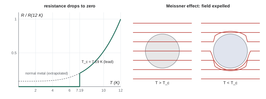
In 1911, Heike Kamerlingh Onnes, who had liquefied helium three years earlier in Leiden, measured the resistance of mercury as he cooled it. At 4.2 K the resistance dropped abruptly to an unmeasurably small value. Lead becomes superconducting at 7.19 K, niobium at 9.25 K, aluminium at 1.18 K. Copper, silver and gold, the best normal conductors, never become superconducting at all. Persistent currents set up in superconducting rings have been observed for years without measurable decay, putting the resistivity below \(10^{-25}\ \Omega\,\text{m}\), at least 17 orders of magnitude below copper's.

The Meissner effect and London theory

Zero resistance alone does not define a superconductor. In 1933, Walther Meissner and Robert Ochsenfeld found that a superconductor cooled in a magnetic field expels the field from its interior. A perfect conductor would merely trap whatever field was present when it became perfect; a superconductor actively pushes it out. This makes the superconducting state a true thermodynamic phase, independent of history, and a perfect diamagnet with \(\chi = -1\). The expulsion is what lets a magnet levitate above a superconductor.

In 1935, the brothers Fritz and Heinz London proposed that the supercurrent density is proportional to the vector potential, \(\mathbf j_s = -(n_se^2/m)\mathbf A\), where \(n_s\) is the density of superconducting electrons. Taking the curl and combining with Ampère's law, \(\nabla\times\mathbf B = \mu_0\mathbf j_s\), gives

The field decays exponentially into the superconductor over the London penetration depth \(\lambda_L\). Using the free-electron density for \(n_s\), the program finds 12 to 23 nm for common superconductors, compared with measured values of 16 to 39 nm; the agreement is fair for aluminium and worse for the others, where the nonlocal response of the electron pairs, with sizes larger than \(\lambda_L\), increases the effective penetration. The London equation also explains why the supercurrent flows only in a thin surface layer.

Superconductivity is destroyed by a strong enough field. In type I superconductors, such as lead, the field is expelled up to a critical field \(B_c(T) \approx B_c(0)[1 - (T/T_c)^2]\), 80 mT for lead, and then penetrates completely. In type II superconductors, including niobium and the alloys used in magnets, the field enters above a lower critical field as an array of quantized flux tubes, each carrying one flux quantum \(\Phi_0 = h/2e = 2.07 \times 10^{-15}\) Wb, and superconductivity survives up to an upper critical field that can exceed 10 T. Alexei Abrikosov predicted these vortices in 1957. The factor \(2e\) in the flux quantum is a crucial clue: the charge carriers are pairs of electrons.

BCS theory

The microscopic explanation came in 1957 from John Bardeen, Leon Cooper and Robert Schrieffer. Its key ingredients are already in this course. In 1950, the isotope effect showed that \(T_c\) depends on the mass of the ions, roughly \(T_c \propto M^{-1/2}\), proving that lattice vibrations are involved. The physical picture is that an electron passing through the lattice attracts the positive ions, leaving a slight concentration of positive charge in its wake that attracts a second electron. Because the ions are slow, the attraction is retarded and can outweigh the Coulomb repulsion for electrons within about a phonon energy \(k_B\theta_D\) of the Fermi surface.

Cooper showed in 1956 that any attraction, however weak, binds two electrons just above a filled Fermi sea into a pair with opposite momenta and spins, because the Fermi sea blocks them from scattering into lower states, the Pauli principle of lesson 7. In the BCS ground state, all electrons near the Fermi surface form such Cooper pairs, and the pairs, being bosons in a sense, occupy one coherent quantum state described by a single macroscopic wave function. Breaking a pair costs at least \(2\Delta\), where \(\Delta\) is the energy gap. BCS theory predicts

a universal ratio for weak coupling. The program compares it with measured gaps. Aluminium and tin agree closely; lead and niobium, with stronger electron–phonon coupling, have somewhat larger gaps, consistent with extensions of the theory. The gap explains the exponential decrease of the electronic heat capacity below \(T_c\) and the absorption of far-infrared radiation only above \(2\Delta\). Because scattering a pair would require breaking it or changing the state of all pairs together, small impurities and phonons cannot slow the condensate, and current flows without resistance. The pair size, the coherence length, is typically 100 to 1000 nm in elemental superconductors, so millions of pairs overlap. Brian Josephson predicted in 1962 that pairs tunnel through a thin barrier between two superconductors, producing the Josephson effects used in SQUID magnetometers and superconducting qubits, the work recognized by the 2025 Nobel Prize in Physics to John Clarke, Michel Devoret and John Martinis.

High-temperature superconductors and applications

Until 1986, the highest known \(T_c\), reached in 1973 in niobium–germanium, was about 23 K. In 1986, J. Georg Bednorz and K. Alex Müller at IBM Zurich found superconductivity near 35 K in a lanthanum–barium–copper oxide, and within a year yttrium–barium–copper oxide was found to superconduct at 93 K, above the boiling point of liquid nitrogen. The copper oxides are layered materials whose parent compounds are Mott insulators, and their pairing mechanism is still debated. Magnesium diboride (39 K, 2001) and iron-based superconductors (up to about 55 K, 2008) followed. Hydrogen-rich compounds such as \(\text{H}_3\text{S}\) superconduct above 200 K, but only under pressures above a million atmospheres. Claims of room-temperature superconductivity at ambient pressure have so far not survived checking: the copper-doped lead apatite called LK-99, announced in 2023, was quickly shown by many groups to be an insulator whose apparent levitation came from ferromagnetic impurities.

Applications use mainly niobium–titanium (\(T_c \approx 9\) K) and niobium–tin cooled by liquid helium. The magnets of MRI scanners, about 1.5 or 3 T, the 1232 dipole magnets of the Large Hadron Collider, at 8.3 T, and many research magnets are wound from these wires. Copper oxide tapes are entering use in power cables, fault-current limiters and compact high-field magnets for fusion research.

Graphene

Graphene is a single layer of carbon atoms in a honeycomb pattern, the building block of graphite. Andre Geim and Konstantin Novoselov isolated it in 2004 by peeling layers from graphite with adhesive tape, and shared the 2010 Nobel Prize in Physics. The honeycomb is not a Bravais lattice; it is a hexagonal lattice with a two-atom basis, the two atoms labelled A and B. Each carbon atom forms three in-plane bonds, and the remaining \(p_z\) orbital, perpendicular to the plane, forms the \(\pi\) bands that control the electronic properties.

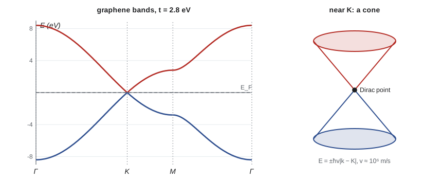
A tight-binding model with one \(p_z\) orbital on each of the two sublattices, hopping \(t \approx 2.8\) eV between closest atoms, gives a \(2 \times 2\) problem like that of the diatomic chain in lesson 5. Its solution is

where \(\boldsymbol\delta_j\) are the three vectors from an A atom to its B neighbours. The two bands are symmetric about zero energy. With one \(\pi\) electron per atom, the lower band is exactly full. At the corners \(K\) of the hexagonal Brillouin zone of lesson 3, the sum of the three phase factors vanishes, so the bands touch. Near \(K\), they are linear,

where \(a_{cc} = 0.142\) nm is the carbon–carbon distance. This is the energy–momentum relation of a massless relativistic particle, with the speed of light replaced by \(v_F\), about \(c/300\): the electrons of graphene obey a two-dimensional Dirac equation. Graphene is neither a metal nor an insulator but a semimetal with zero gap and a Fermi surface shrunk to points. Its carriers are extremely mobile, it conducts heat superbly, and it absorbs a fraction \(\pi\alpha \approx 2.3\) parts in 100 of visible light per layer, set by the fine-structure constant.

import math
# Superconductivity scales, then the graphene band structure.
e, me, mu0, kB, hbar = 1.602176634e-19, 9.1093837e-31, 4e-7 * math.pi, 1.380649e-23, 1.054571817e-34
print("London penetration depth lambda = sqrt(m / (mu0 n e^2)) for the free-electron density")
for name, n, meas in (("Al", 18.1e28, 16), ("Sn", 14.8e28, 34), ("Pb", 13.2e28, 37), ("Nb", 5.56e28, 39)):
    lam = math.sqrt(me / (mu0 * n * e * e))
    print(f"   {name}: n = {n:.2e} per m^3, lambda_L = {lam * 1e9:5.1f} nm (measured about {meas} nm)")
print()
print("BCS weak-coupling gap Delta(0) = 1.764 kB Tc")
for name, Tc, meas in (("Al", 1.18, 0.18), ("Sn", 3.72, 0.59), ("Pb", 7.19, 1.36), ("Nb", 9.25, 1.55)):
    D = 1.764 * kB * Tc / e * 1e3
    print(f"   {name}: Tc = {Tc:5.2f} K, BCS Delta = {D:.3f} meV, measured about {meas:.2f} meV,"
          f" ratio 2Delta/kTc measured = {2 * meas * 1e-3 * e / (kB * Tc):.2f}")
Hc0, Tc = 0.0803, 7.19   # lead, tesla
print("critical field of lead, Bc(T) = Bc(0) [1 - (T/Tc)^2]:",
      ", ".join(f"{T} K {Hc0 * (1 - (T / Tc) ** 2) * 1e3:.1f} mT" for T in (0, 2, 4, 6, 7)))
print()
# Graphene: tight binding on a honeycomb lattice, t = 2.8 eV, C-C distance 0.142 nm
t, acc = 2.8, 0.142e-9
def bands(kx, ky):
    # vectors from an A atom to its three closest B atoms
    d = [(acc, 0.0), (-acc / 2, acc * math.sqrt(3) / 2), (-acc / 2, -acc * math.sqrt(3) / 2)]
    f = sum(complex(math.cos(kx * dx + ky * dy), math.sin(kx * dx + ky * dy)) for dx, dy in d)
    return -t * abs(f), t * abs(f)
K = (2 * math.pi / (3 * acc), 2 * math.pi / (3 * math.sqrt(3) * acc))
G = (0.0, 0.0)
print(f"graphene: at Gamma the bands are at {bands(*G)[0]:+.2f} and {bands(*G)[1]:+.2f} eV")
print(f"          at K they touch: {bands(*K)[0]:+.4f} and {bands(*K)[1]:+.4f} eV (a Dirac point)")
dk = 1e7
Eup = bands(K[0] + dk, K[1])[1]
vF = Eup * e / (hbar * dk)
print(f"          slope near K gives v = {vF:.3e} m/s; formula 3 t a_cc / (2 hbar) = {3 * t * e * acc / (2 * hbar):.3e} m/s"
      f" (about c/{2.998e8 / vF:.0f})")

London penetration depth lambda = sqrt(m / (mu0 n e^2)) for the free-electron density
   Al: n = 1.81e+29 per m^3, lambda_L =  12.5 nm (measured about 16 nm)
   Sn: n = 1.48e+29 per m^3, lambda_L =  13.8 nm (measured about 34 nm)
   Pb: n = 1.32e+29 per m^3, lambda_L =  14.6 nm (measured about 37 nm)
   Nb: n = 5.56e+28 per m^3, lambda_L =  22.5 nm (measured about 39 nm)

BCS weak-coupling gap Delta(0) = 1.764 kB Tc
   Al: Tc =  1.18 K, BCS Delta = 0.179 meV, measured about 0.18 meV, ratio 2Delta/kTc measured = 3.54
   Sn: Tc =  3.72 K, BCS Delta = 0.565 meV, measured about 0.59 meV, ratio 2Delta/kTc measured = 3.68
   Pb: Tc =  7.19 K, BCS Delta = 1.093 meV, measured about 1.36 meV, ratio 2Delta/kTc measured = 4.39
   Nb: Tc =  9.25 K, BCS Delta = 1.406 meV, measured about 1.55 meV, ratio 2Delta/kTc measured = 3.89
critical field of lead, Bc(T) = Bc(0) [1 - (T/Tc)^2]: 0 K 80.3 mT, 2 K 74.1 mT, 4 K 55.4 mT, 6 K 24.4 mT, 7 K 4.2 mT

graphene: at Gamma the bands are at -8.40 and +8.40 eV
          at K they touch: -0.0000 and +0.0000 eV (a Dirac point)
          slope near K gives v = 9.061e+05 m/s; formula 3 t a_cc / (2 hbar) = 9.061e+05 m/s (about c/331)

The program confirms the band structure: \(\pm8.4\) eV at \(\Gamma\), equal to \(\pm3t\); exact touching at \(K\); and a slope near \(K\) giving \(v_F = 9.1 \times 10^5\) m/s, matching the formula and within about 10 parts in 100 of measured values.

Topological insulators and quantum materials

Band theory, as developed in lessons 8 and 9, classifies materials by whether bands are full or empty. In the 1980s it emerged that bands carry a second kind of information: a topological invariant, an integer that describes how the Bloch wave functions twist across the Brillouin zone and that cannot change without closing the gap. David Thouless and coworkers showed in 1982 that this integer is the quantized Hall conductance of the quantum Hall effect, and Duncan Haldane showed in 1988 that it can be nonzero even without a magnetic field. Thouless, Haldane and Michael Kosterlitz shared the 2016 Nobel Prize in Physics for topological phases of matter.

In 2005, Charles Kane and Eugene Mele showed that strong spin–orbit coupling in graphene-like systems could produce a time-reversal-invariant topological insulator: insulating inside, but with conducting states along its edges that cannot be removed by any perturbation preserving time-reversal symmetry. The idea extends to three dimensions, where the boundary carries conducting surface states with Dirac-cone dispersion like graphene's. Photoemission confirmed three-dimensional topological insulators in bismuth–antimony alloys in 2008 and in bismuth selenide and bismuth telluride in 2009. The same ideas now classify superconductors, semimetals and even phonon and photon bands.

The frontier of the field, often called quantum materials, includes twisted bilayer graphene, which becomes superconducting when two sheets are rotated by about 1.1 degrees relative to each other (2018); heavy-fermion compounds; quantum spin liquids, in which frustrated magnetic moments refuse to order; and materials designed atom by atom by stacking two-dimensional layers. Each builds on the concepts of this course: lattices and reciprocal space, bands and their filling, phonons and their coupling to electrons, and the exchange and pairing that arise from the Pauli principle.