Magnetism in solids: diamagnetism, paramagnetism and ferromagnetism

Every material responds to a magnetic field, but the responses differ enormously in size and sign. Copper and water are weakly repelled by a magnet; aluminium and liquid oxygen are weakly attracted; iron, nickel and cobalt are attracted strongly and can stay magnetized after the field is removed. PHYS-381 described magnetic materials through the magnetization \(\mathbf M\), the field \(\mathbf H\) and the susceptibility \(\chi = M/H\). This lesson explains where those responses come from at the atomic level. Magnetism turns out to be a purely quantum phenomenon: the Bohr–van Leeuwen theorem, proved in 1911 and 1919, shows that classical statistical mechanics gives zero magnetization in thermal equilibrium. Every magnetic effect in solids comes from electron spin, orbital angular momentum and the Pauli principle.

Magnetic moments and susceptibility

The natural unit of atomic magnetism is the Bohr magneton, \(\mu_B = e\hbar/2m = 9.274 \times 10^{-24}\ \text{J/T}\), the moment associated with one unit of orbital angular momentum. An electron's spin moment is \(g\mu_BS\) with \(g \approx 2.0023\), as PHYS-373 showed. Atoms with completely filled shells have zero net spin and orbital angular momentum and therefore no permanent moment; atoms or ions with partly filled shells, such as the \(3d\) transition-metal ions and the \(4f\) rare-earth ions, do. Hund's rules, also from PHYS-373, predict the ground-state spin and orbital angular momentum of such ions and so their moments. The dimensionless susceptibility in SI units is \(\chi = \mu_0M/B\) for small fields. Materials with \(\chi < 0\) are diamagnetic; those with small \(\chi > 0\) are paramagnetic; ferromagnets have enormous, field-dependent effective susceptibilities and spontaneous magnetization.

Diamagnetism

Every material has a diamagnetic contribution. An applied field changes the orbital motion of the electrons in each atom, inducing a current that opposes the field, much as Lenz's law requires. Quantum mechanics gives the Langevin (or Larmor) susceptibility,

where \(n\) is the number of atoms per unit volume and \(\langle r^2\rangle\) the mean square radius of each electron's orbit. For typical solids \(\chi_{dia} \sim -10^{-5}\), independent of temperature. It is usually swamped by other contributions, but it dominates in materials with only filled shells, such as the noble gases, most organic compounds and water. With a field gradient strong enough, diamagnetic repulsion can balance gravity: Andre Geim levitated a live frog in a 16 T magnet in 1997, and won an Ig Nobel Prize for it before his Nobel Prize for graphene. Superconductors, in lesson 12, are perfect diamagnets with \(\chi = -1\).

Paramagnetism

When atoms carry permanent moments that interact only weakly with each other, an applied field tends to align them while thermal agitation randomizes them. For spin one-half, each moment has two energy levels, \(\mp\mu_BB\), and the Boltzmann distribution from PHYS-361 gives an average moment \(\mu_B\tanh(\mu_BB/k_BT)\). For \(\mu_BB \ll k_BT\), which holds except in strong fields at low temperature, \(\tanh x \approx x\), and

Curie's law, found experimentally by Pierre Curie in 1895. For a general angular momentum \(J\), the constant becomes \(C = \mu_0ng^2J(J + 1)\mu_B^2/3k_B\), and the full field dependence is given by the Brillouin function. The program shows that a dilute paramagnet with \(10^{28}\) moments per cubic metre has \(\chi \approx 2.6 \times 10^{-4}\) at room temperature, rising a hundredfold by 3 K. Paramagnetic salts at very low temperature are used to cool samples further, by adiabatic demagnetization, reaching millikelvin temperatures.

Conduction electrons in a metal also have spin moments, but they do not follow Curie's law. Because the electron gas is degenerate, only electrons within about \(k_BT\) of the Fermi energy can flip their spins, as with the heat capacity in lesson 7. Wolfgang Pauli showed in 1927 that the resulting spin susceptibility is temperature-independent and of order

about \(10^{-5}\) for copper, as the program shows. In copper the core-electron diamagnetism is larger, so copper is weakly diamagnetic overall; in sodium and aluminium Pauli paramagnetism wins, and they are weakly paramagnetic.

Ferromagnetism and the exchange interaction

In iron, cobalt and nickel, and in many compounds, the moments align spontaneously below a critical temperature \(T_c\), called the Curie temperature: 1043 K for iron, 1388 K for cobalt, 627 K for nickel. What aligns them? Not their magnetic dipole fields. The program estimates that the dipole field of one Bohr magneton at a typical spacing of 0.25 nm is about 0.06 T, which could align moments only below about 0.04 K. The field that would be needed to align moments against thermal agitation at iron's Curie temperature is more than 1000 T, far beyond any magnet.

Werner Heisenberg identified the cause in 1928: the exchange interaction. As PHYS-373 showed for helium, the Pauli principle couples the spatial symmetry of a two-electron wave function to its spin state, so the Coulomb repulsion between electrons depends on their relative spin orientation, even though the repulsion itself contains no spin. The energy difference can be written as an effective coupling between spins,

the Heisenberg model, where \(J_{ij}\) is the exchange constant between neighbouring spins. If \(J > 0\), parallel spins are favoured and the material can become a ferromagnet; if \(J < 0\), antiparallel neighbours are favoured, giving an antiferromagnet such as manganese oxide or chromium, in which alternate moments point in opposite directions and the net magnetization vanishes. Exchange energies are electrostatic in origin and of order 0.01 to 0.1 eV, which is why magnetic ordering can survive to hundreds of kelvin. In metals such as iron, the exchange acts between itinerant \(d\) electrons, and a band picture of ferromagnetism, due to Edmund Stoner, is more appropriate: the spin-up and spin-down bands split, and the moment per atom is a non-integer number of Bohr magnetons, 2.2 for iron and 0.6 for nickel.

Mean-field theory

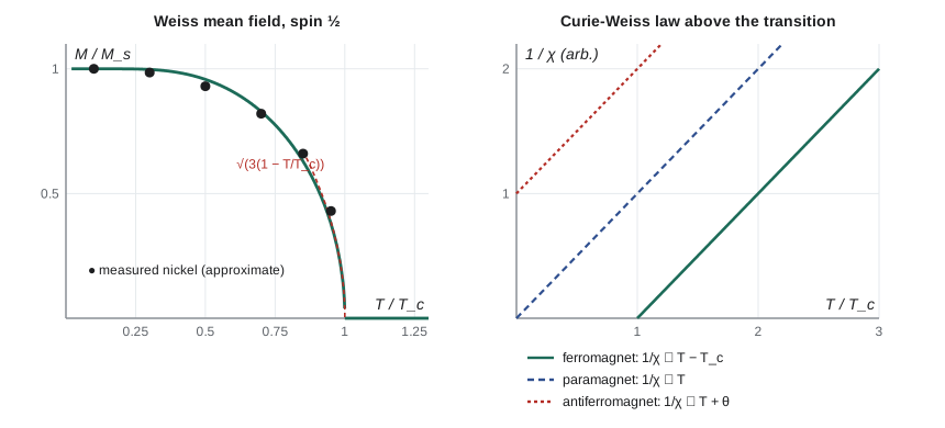
Pierre Weiss proposed in 1907, long before the quantum explanation, that each moment feels an internal molecular field proportional to the magnetization, \(B_{mf} = \lambda M\). In the Heisenberg model this is a mean-field approximation: replace the neighbours' spins by their average. For spin one-half, each moment then sees a total field \(B + \lambda M\), and the paramagnetic result becomes self-consistent:

where \(T_c = \lambda\mu_0 n\mu_B^2/k_B\) in terms of Weiss's constant. This equation always has the solution \(m = 0\). Below \(T_c\) it also has nonzero solutions \(\pm m\), with lower free energy: spontaneous magnetization. The program solves it by iteration. Near \(T_c\), expanding \(\tanh x \approx x - x^3/3\) gives \(m \approx \sqrt{3(1 - T/T_c)}\), which the numbers confirm. Above \(T_c\), the mean-field susceptibility becomes

the Curie–Weiss law, which diverges as \(T\) approaches \(T_c\) from above. For an antiferromagnet, \(\chi = C/(T + \theta)\) with \(\theta > 0\). Plots of \(1/\chi\) against \(T\) above the transition distinguish the cases by their intercepts.

import math
# Magnetism: Curie paramagnet, Weiss mean field for a ferromagnet, and two diamagnetic scales.
kB, muB, mu0 = 1.380649e-23, 9.2740101e-24, 4e-7 * math.pi
def mean_field_m(t):
    """Spin one-half Weiss model: m = tanh(m / t), t = T / Tc. Returns the positive root."""
    if t >= 1: return 0.0
    m = 1.0
    for _ in range(2000):
        m_new = math.tanh(m / t)
        if abs(m_new - m) < 1e-14: break
        m = m_new
    return m
print("Weiss mean field, spin 1/2: reduced magnetization m(T/Tc)")
for t in (0.1, 0.3, 0.5, 0.7, 0.9, 0.95, 0.99, 1.0, 1.1):
    m = mean_field_m(t)
    near = f"   sqrt(3(1 - t)) = {math.sqrt(3 * (1 - t)):.4f}" if 0.9 <= t < 1 else ""
    print(f"   T/Tc = {t:4.2f}: m = {m:.4f}{near}")
print()
# Iron: the molecular field needed to align a moment of one Bohr magneton against kB Tc
Tc = 1043.0
B_mf = kB * Tc / muB
print(f"iron: molecular field implied by Tc = 1043 K is about {B_mf:.0f} T, far beyond laboratory magnets;"
      " its origin is the exchange interaction, not dipole fields")
B_dip = mu0 * muB / (4 * math.pi * (0.25e-9) ** 3)
print(f"dipole field of one Bohr magneton at 0.25 nm: {B_dip:.2f} T, ordering temperature ~ {muB * B_dip / kB:.2f} K")
print()
# Curie law for a dilute spin-1/2 paramagnet, n = 1e28 per m^3
n = 1e28
C = mu0 * n * muB ** 2 / kB
for T in (1, 4.2, 77, 300):
    print(f"   Curie susceptibility at {T:5.1f} K: chi = {C / T:.2e}")
# Pauli paramagnetism of copper electrons and Langevin diamagnetism scale
EF = 7.0 * 1.602176634e-19; ne = 8.47e28
chi_P = mu0 * muB ** 2 * 3 * ne / (2 * EF)
print(f"Pauli spin susceptibility of the copper electron gas: {chi_P:.2e} (temperature independent)")
print("measured total for copper is about -1e-5: core-electron diamagnetism wins")

Weiss mean field, spin 1/2: reduced magnetization m(T/Tc)
   T/Tc = 0.10: m = 1.0000
   T/Tc = 0.30: m = 0.9974
   T/Tc = 0.50: m = 0.9575
   T/Tc = 0.70: m = 0.8286
   T/Tc = 0.90: m = 0.5254   sqrt(3(1 - t)) = 0.5477
   T/Tc = 0.95: m = 0.3795   sqrt(3(1 - t)) = 0.3873
   T/Tc = 0.99: m = 0.1725   sqrt(3(1 - t)) = 0.1732
   T/Tc = 1.00: m = 0.0000
   T/Tc = 1.10: m = 0.0000

iron: molecular field implied by Tc = 1043 K is about 1553 T, far beyond laboratory magnets; its origin is the exchange interaction, not dipole fields
dipole field of one Bohr magneton at 0.25 nm: 0.06 T, ordering temperature ~ 0.04 K

   Curie susceptibility at   1.0 K: chi = 7.83e-02
   Curie susceptibility at   4.2 K: chi = 1.86e-02
   Curie susceptibility at  77.0 K: chi = 1.02e-03
   Curie susceptibility at 300.0 K: chi = 2.61e-04
Pauli spin susceptibility of the copper electron gas: 1.22e-05 (temperature independent)
measured total for copper is about -1e-5: core-electron diamagnetism wins

Mean-field theory captures the existence of the transition and the shape of \(M(T)\) qualitatively, but it is not exact. Near \(T_c\), measured magnetizations fall as \((1 - T/T_c)^\beta\) with \(\beta \approx 0.33\) to \(0.37\) for three-dimensional magnets, not the mean-field \(\tfrac12\). At low temperature, the magnetization falls as \(T^{3/2}\) rather than exponentially, because of collective spin waves, called magnons, the magnetic analogue of phonons, which Bloch introduced in 1930 and Brockhouse measured with neutrons in 1957. In one dimension, fluctuations destroy ordering altogether at any nonzero temperature. Getting the critical behaviour right required the renormalization group, for which Kenneth Wilson received the 1982 Nobel Prize, and the exact solution of the two-dimensional Ising model by Lars Onsager in 1944, which PHYS-361 discusses.

Domains and hysteresis

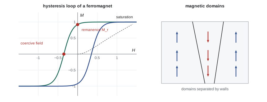
If iron is spontaneously magnetized below 1043 K, why is an ordinary iron nail not a magnet? Weiss again supplied the answer: a ferromagnet divides into domains, regions each magnetized to saturation but in different directions, so that the overall magnetization is small. Domains form because a uniformly magnetized block creates a large external field storing magnetic energy; breaking into domains with closed flux paths lowers that energy, at the cost of creating domain walls, transition layers tens of nanometres thick in iron, where the moments rotate gradually.

Applying a field makes favourably oriented domains grow at the expense of others, by moving walls, and finally rotates the moments into alignment. Walls get pinned at defects and grain boundaries, so the process is irreversible and the magnetization curve shows hysteresis. The remanence is the magnetization left when the field returns to zero; the coercive field is the reverse field needed to bring it back to zero. Soft magnetic materials, such as silicon steel in transformer cores, have narrow loops and lose little energy per cycle. Hard materials, such as the neodymium–iron–boron magnets developed in 1982–84 and used in electric-vehicle motors and wind turbines, have wide loops with coercive fields above 1 T, so they keep their magnetization against demagnetizing fields.

Magnetic storage relies on the same physics. A hard-disk platter stores each bit in a tiny region of a cobalt alloy film, whose orientation is read using giant magnetoresistance, a change of resistance with the relative alignment of magnetic layers, discovered independently by Albert Fert and Peter Grünberg in 1988 and recognized with the 2007 Nobel Prize in Physics.