Classic experiments II: photoelectric effect, Franck–Hertz and Planck's constant

Two experiments of the early twentieth century made the quantum unavoidable. The photoelectric effect showed that light delivers its energy in lumps proportional to its frequency, and gave a direct measurement of Planck's constant. The Franck–Hertz experiment showed that atoms absorb energy from colliding electrons only in definite amounts, confirming that atomic energy levels are discrete. PHYS-271 presented these results as part of the story of modern physics. This lesson looks at them as experiments: what is actually measured, what can go wrong, and how to extract \(h\) and an excitation energy from real-looking data with honest uncertainties.

The photoelectric effect

Heinrich Hertz noticed in 1887 that ultraviolet light made sparks jump more easily between electrodes. Philipp Lenard showed around 1902 that light ejects electrons from metal surfaces, and found a puzzle: the maximum energy of the ejected electrons did not depend on the intensity of the light, only on its frequency, and below a threshold frequency no electrons emerged at all, however bright the light. In 1905 Albert Einstein proposed that light itself consists of quanta of energy \(hf\). An electron absorbs a single quantum and escapes with at most the energy left after paying the work function \(W\) of the surface:

This explained everything Lenard saw: more intense light means more photons and more electrons, but not more energetic ones, and photons with \(hf < W\) cannot free any electron. It also made a bold prediction: a graph of \(K_{\max}\) against \(f\) should be a straight line with slope \(h\), the same for every metal. Robert Millikan, who doubted the photon idea, spent a decade testing it, and in 1916 published measurements that confirmed the linear relation and gave \(h\) to within about half a part in 100. Einstein's Nobel Prize of 1921 was awarded for this law, and Millikan's of 1923 in part for testing it.

Measuring the stopping potential

In the teaching version, light from a mercury lamp passes through a filter or monochromator that selects one spectral line and falls on a photocathode in a vacuum tube. Electrons ejected from the cathode travel to an anode. A retarding voltage applied to the anode repels them, and the photocurrent falls as the voltage rises. At the stopping potential \(V_s\), even the fastest electrons are turned back and the current drops to zero:

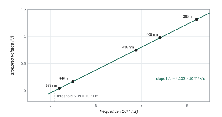
A plot of \(V_s\) against \(f\) has slope \(h/e\) and intercept \(-W/e\). Mercury lamps are convenient because their bright lines at 365.0, 404.7, 435.8, 546.1 and 577.0 nm span a factor of 1.6 in frequency. Several experimental problems make the measurement harder than the equation suggests. The current near the stopping potential approaches zero gradually rather than abruptly, because the electrons have a spread of energies, so locating \(V_s\) needs a definite criterion applied the same way at every wavelength. Light scattered onto the anode ejects electrons from it, giving a small reverse current that masks the true zero. The anode and cathode are made of different metals, so a contact potential of order a volt adds to the applied voltage. This last effect shifts the intercept and so the apparent work function, but not the slope, which is why \(h\) can be measured well even when \(W\) cannot.

Fitting the data, and an honest uncertainty

The program simulates the five mercury lines on a cathode whose effective work function, including contact potential, is 2.10 eV, with a reading uncertainty of 0.02 V on each stopping voltage. It fits a straight line, then estimates the uncertainty of the slope in two ways: from the known reading uncertainty, and from the scatter of the points about the line.

import math, random
random.seed(397)
h_true, e, c = 6.62607015e-34, 1.602176634e-19, 299792458.0
# 1. Photoelectric effect with the mercury lines; cathode work function about 2.10 eV (plus contact potential).
lines_nm = [365.0, 404.7, 435.8, 546.1, 577.0]
W = 2.10
data = []
for lam in lines_nm:
    f = c/(lam*1e-9)
    Vs = h_true*f/e - W + random.gauss(0, 0.02)       # stopping voltage, 0.02 V reading uncertainty
    data.append((f, Vs))
n = len(data); mf = sum(f for f, _ in data)/n; mv = sum(v for _, v in data)/n
Sff = sum((f - mf)**2 for f, _ in data); slope = sum((f - mf)*(v - mv) for f, v in data)/Sff
icpt = mv - slope*mf
res = [v - (icpt + slope*f) for f, v in data]
s = math.sqrt(sum(r*r for r in res)/(n - 2))
h = slope*e; dh = 0.02/math.sqrt(Sff)*e; dh_res = s/math.sqrt(Sff)*e
chi2 = sum((r/0.02)**2 for r in res)
print("frequency (1e14 Hz) and stopping voltage (V):", ", ".join(f"{f/1e14:.3f}: {v:.3f}" for f, v in data))
print(f"h = {h:.4e} +/- {dh:.1e} J s from the 0.02 V reading uncertainty (accepted 6.6261e-34)")
print(f"   the residual scatter alone would suggest +/- {dh_res:.1e}; chi-squared = {chi2:.2f} for 3 dof")
print(f"work function = {-icpt:.3f} eV; threshold frequency {-icpt*e/h/1e14:.3f}e14 Hz")
# 2. Franck-Hertz curve for mercury: collector current versus accelerating voltage.
Eexc, Vc = 4.89, 2.1          # first excitation energy (eV) and contact potential offset (V)
def current(V):
    x = V - Vc
    if x <= 0: return 0.0
    k = math.floor(x/Eexc); r = x - k*Eexc           # energy left after k inelastic collisions
    return (x**1.5)*(0.25 + 0.75*(1 - math.exp(-r/0.9)))*math.exp(-0.04*k)
Vs = [i*0.05 for i in range(0, 601)]
I = [current(V) + random.gauss(0, 0.05) for V in Vs]
sm = [sum(I[max(0, i - 3):i + 4])/len(I[max(0, i - 3):i + 4]) for i in range(len(I))]   # 7-point smoothing
peaks = [Vs[i] for i in range(10, len(sm) - 10) if sm[i] == max(sm[i - 10:i + 11]) and Vs[i] > 4]
print("peak voltages (V):", ", ".join(f"{p:.2f}" for p in peaks))
sp = [b - a for a, b in zip(peaks, peaks[1:])]
print(f"mean spacing {sum(sp)/len(sp):.2f} V -> excitation energy {sum(sp)/len(sp):.2f} eV, photon wavelength {h_true*c/(sum(sp)/len(sp)*e)*1e9:.0f} nm")

frequency (1e14 Hz) and stopping voltage (V): 8.213: 1.311, 7.408: 0.977, 6.879: 0.745, 5.490: 0.169, 5.196: 0.043
h = 6.7327e-34 +/- 1.3e-35 J s from the 0.02 V reading uncertainty (accepted 6.6261e-34)
   the residual scatter alone would suggest +/- 2.8e-36; chi-squared = 0.14 for 3 dof
work function = 2.140 eV; threshold frequency 5.092e14 Hz
peak voltages (V): 6.80, 11.70, 16.60, 21.50, 26.35
mean spacing 4.89 V -> excitation energy 4.89 eV, photon wavelength 254 nm

The fit gives \(h = (6.73 \pm 0.13) \times 10^{-34}\) J s when the uncertainty is based on the known 0.02 V reading error, in agreement with the accepted \(6.626 \times 10^{-34}\) J s at 0.8 standard uncertainties. Now look at what happens with the other estimate. By chance, the five points lie unusually close to the line, so the residual scatter suggests an uncertainty five times smaller, \(\pm 0.028 \times 10^{-34}\), which would make the result appear to disagree with the accepted value by almost four standard uncertainties. The chi-squared of 0.14 for three degrees of freedom flags the problem: it is improbably small. With only five points and two parameters, the scatter is a poor estimate of the true uncertainty. When you know the measurement uncertainty from the instrument and the method, use it, and use chi-squared to check it; do not replace a well-founded uncertainty with the scatter of a handful of points.

The Franck–Hertz experiment

In 1914 James Franck and Gustav Hertz, a nephew of Heinrich, accelerated electrons through mercury vapour and measured how many reached a collector. Electrons leave a heated cathode, are accelerated toward a grid by a voltage \(V\), and those that pass the grid must overcome a small retarding voltage, about half a volt, to reach the collector. Plotting collector current against accelerating voltage, Franck and Hertz saw the current rise, then drop sharply at intervals of about 4.9 V, rise again, drop again, in a series of regularly spaced peaks.

The explanation is that a mercury atom can absorb energy from a colliding electron only if the electron has at least 4.9 eV, the energy of the atom's first excited state. Below that, collisions are elastic: a light electron bouncing off a heavy atom loses almost no energy. When the accelerating voltage reaches 4.9 V, electrons gain enough energy just in front of the grid to excite an atom, lose almost all their energy, and can no longer climb the retarding voltage: the current drops. Raise the voltage further and the electrons gain 4.9 eV well before the grid, lose it, and are reaccelerated; at 9.8 V they can excite two atoms in succession, and so on. The spacing of the peaks measures the excitation energy directly. Franck and Hertz also saw the excited mercury atoms emit ultraviolet light at 253.7 nm, the wavelength corresponding to 4.89 eV, confirming the interpretation. They shared the Nobel Prize in 1925. The experiment was the first direct evidence for Niels Bohr's discrete atomic energy levels, proposed in 1913, although Franck and Hertz at first interpreted their result as ionization.

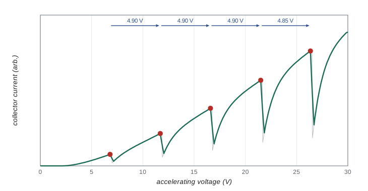
Two details matter in practice. The first peak is not at 4.9 V but higher, because the contact potential between the cathode and grid adds to the applied voltage; the spacing between peaks is unaffected, which is why it, not the position of the first peak, is the measured quantity. And the peaks are rounded, not sharp, because the electrons leave the cathode with a spread of thermal energies and because some electrons excite higher levels. Measuring all the peak positions and fitting them against peak number gives the spacing with an uncertainty, and checks that it is constant. The simulated curve, with a contact potential of 2.1 V and noise added, gives peaks at 6.80, 11.70, 16.60, 21.50 and 26.35 V, a mean spacing of 4.89 V, and a predicted emission wavelength of 254 nm. Smoothing over seven points before finding the peaks prevents noise from producing false maxima; a more careful analysis would fit a smooth function near each peak.

Planck's constant then and now

Max Planck introduced \(h\) in 1900 to explain the spectrum of blackbody radiation, as a mathematical device he hoped to remove. The photoelectric effect and spectroscopy made it physical. Its value was measured by many methods over the century: the photoelectric effect, X-ray spectra, the Josephson effect in superconductors and the watt balance, now called the Kibble balance after Bryan Kibble, which compares mechanical and electrical power so precisely that it could weigh a kilogram in terms of \(h\). The National Research Council of Canada's Kibble balance made one of the most precise measurements, with an uncertainty of about 9 parts in a billion, and contributed to fixing \(h = 6.62607015 \times 10^{-34}\) J s exactly in the 2019 redefinition of the kilogram. A student photoelectric measurement good to 2 parts in 100 is part of the same story.