Electronics for physicists II: amplifiers, filters, op-amps and signal-to-noise

Signals from sensors are often tiny: microvolts from a thermocouple, nanoamperes from a photodiode in dim light, femtocoulombs from a particle detector. To measure them, we amplify them, filter away frequencies that carry only noise, and understand the fundamental noise that no amount of care can remove. This lesson builds the three tools that do this: the RC filter and its frequency response, the operational amplifier with negative feedback, and the theory of noise, especially the thermal noise of resistors predicted by Harry Nyquist and measured by John Bertrand Johnson in 1928. Its central quantity is the signal-to-noise ratio, which ultimately decides what an experiment can detect.

The RC low-pass filter

Put a resistor \(R\) in series with the signal and a capacitor \(C\) from the output to ground. This is a voltage divider made of impedances, so its transfer function, the ratio of output to input, is

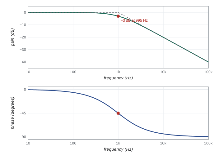
At frequencies well below the corner frequency \(f_c\), the capacitor's impedance is large and the signal passes unchanged. Well above it, \(|H| \approx f_c/f\): the output falls by a factor of ten for every tenfold increase in frequency. At \(f_c\) itself, \(|H| = 1/\sqrt{2}\), half the power, and the output lags the input by 45 degrees. In the time domain the same circuit has time constant \(\tau = RC\): a sudden step at the input reaches 63 of every 100 parts of its final value after one time constant. A low-pass filter therefore averages the signal over a time of order \(\tau\), smoothing fast fluctuations. Swapping the resistor and capacitor gives a high-pass filter, which blocks slow drifts and DC offsets while passing fast signals.

Decibels and Bode plots

Because gains and frequencies span many orders of magnitude, engineers express gain in decibels, \(20\log_{10}|H|\) for a voltage ratio, and plot it against frequency on a logarithmic axis. This Bode plot, named after Hendrik Bode of Bell Labs, turns the RC filter into two straight lines meeting at the corner: flat at 0 dB below \(f_c\), falling at \(-20\) dB per decade above, with the true curve 3 dB below the corner of the asymptotes. A second plot shows phase. Bode plots make it easy to read off bandwidth, roll-off and phase shift, and to combine stages: gains in decibels simply add.

The operational amplifier

An operational amplifier is a high-gain differential amplifier: its output is \(A(V_+ - V_-)\), where the open-loop gain \(A\) may exceed \(10^5\) at low frequencies and the inputs draw almost no current. On its own, this huge and poorly controlled gain is useless. Its power comes from negative feedback, the idea Harold Black worked out on the ferry to Bell Labs in 1927: feed a fraction of the output back to the inverting input, and the circuit settles where the difference between the inputs is tiny. For an ideal op-amp, two golden rules then describe any circuit: the output does whatever is needed to make the voltage difference between the inputs zero, and the inputs draw no current.

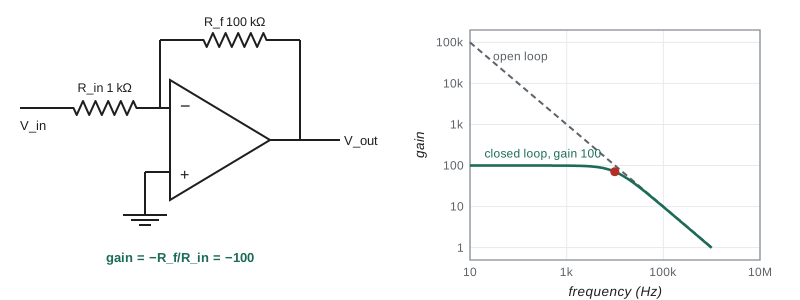
Apply the rules to the inverting amplifier: the input signal reaches the inverting input through \(R_{\text{in}}\), a feedback resistor \(R_f\) connects the output back to that input, and the non-inverting input is grounded. The first rule holds the inverting input at 0 V, a virtual ground. The current through \(R_{\text{in}}\) is therefore \(V_{\text{in}}/R_{\text{in}}\), and by the second rule all of it must flow through \(R_f\), so

The gain depends only on two resistors, which can be stable to a few parts per million per kelvin, not on the op-amp's gain, which may vary by a factor of two between devices. With finite open-loop gain the result is \(G = -(R_f/R_{\text{in}})\,A\beta/(1 + A\beta)\), where \(\beta = R_{\text{in}}/(R_{\text{in}} + R_f)\) is the feedback fraction. The error is about \(1/(A\beta)\). Other standard circuits follow from the same rules: the non-inverting amplifier with gain \(1 + R_f/R_{\text{in}}\) and very high input impedance; the voltage follower, gain 1, used as a buffer to prevent loading; the transimpedance amplifier, which turns a photodiode current \(I\) into a voltage \(-IR_f\); the integrator, with a capacitor in the feedback path.

Gain-bandwidth product

The open-loop gain of a real op-amp is not constant: to keep feedback circuits stable, it is designed to fall at 20 dB per decade above a low corner, often a few hertz, so that gain times frequency is roughly constant. This gain-bandwidth product, typically 1 MHz for a general-purpose device and up to several gigahertz for fast ones, sets a trade-off. An amplifier with a noise gain of 101, the inverse of \(\beta\), has a bandwidth of about \(\text{GBW}/101\), roughly 10 kHz. Need a gain of 10,000 with 100 kHz of bandwidth? A single stage would need a GBW of 1 GHz. Split it into two stages of gain 100; each must hold its gain up to 100 kHz, which needs a GBW of 10 MHz per stage, an ordinary specification. The arithmetic decides which op-amp to buy and how many stages to use.

Noise

Every measurement has noise, random fluctuations added to the signal. Some is interference, which can in principle be removed by shielding and grounding. Some is fundamental. Three kinds dominate in physics laboratories. Johnson–Nyquist noise is the thermal agitation of charge carriers in any resistor at temperature \(T\); Nyquist derived from thermodynamics that its mean square voltage in a bandwidth \(B\) is

independent of the material. A 1 MΩ resistor at room temperature produces 13 μV rms across a 10 kHz bandwidth. Shot noise arises because current is carried by discrete charges arriving at random: for a current \(I\), \(\langle i_n^2\rangle = 2eIB\); it limits photodetectors at low light. Both are white noise, with equal power per unit bandwidth at all frequencies. The third, flicker or \(1/f\) noise, has power that rises at low frequencies, roughly as \(1/f\); it comes from slow fluctuations in materials, contacts and environment, and it is why DC measurements are often noisier than expected. Below a corner frequency, often between 1 Hz and a few kilohertz, \(1/f\) noise dominates.

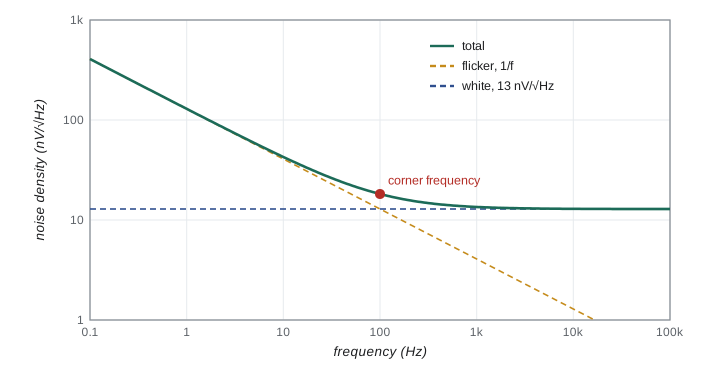
Noise from several independent sources adds in quadrature, like independent uncertainties, so the largest source dominates. A useful way to compare them is to refer every noise to the input of the first amplifier: divide each output noise by the gain that follows it. Op-amp data sheets give an input voltage noise density, typically 1 to 20 nV per root hertz, and an input current noise density, which flows through the source resistance and appears as a voltage. For a low-resistance source such as a thermocouple, the amplifier's voltage noise usually dominates; for a high-resistance source such as a photodiode or a pH electrode, current noise and the Johnson noise of the source dominate. Choosing an amplifier means matching its noise to the source, not simply buying the lowest voltage noise.

Signal-to-noise ratio

The signal-to-noise ratio, the rms signal divided by the rms noise, decides whether a signal can be measured. Because white noise grows as \(\sqrt{B}\), reducing the bandwidth to just what the signal needs improves the ratio. This is the job of filtering, and of averaging, which is a filter in disguise: averaging \(N\) independent samples reduces the noise by \(\sqrt{N}\). Amplification alone never improves the signal-to-noise ratio, because the amplifier amplifies the noise too and adds its own; the first stage of amplification, which sees the smallest signal, matters most, which is why low-noise preamplifiers are placed close to the detector and are sometimes cooled.

import math, cmath
# 1. RC low-pass filter, R = 10 kohm, C = 16 nF: corner frequency and Bode data.
R, C = 10e3, 16e-9
fc = 1/(2*math.pi*R*C)
print(f"corner frequency fc = {fc:.0f} Hz")
for f in (10, 100, fc, 1000, 10000, 100000):
    H = 1/(1 + 1j*2*math.pi*f*R*C)
    print(f"  f = {f:9.0f} Hz: gain {round(20*math.log10(abs(H)), 2) + 0.0:7.2f} dB, phase {math.degrees(cmath.phase(H)):7.1f} degrees")
# 2. Inverting amplifier, Rf = 100 kohm, Rin = 1 kohm, with finite open-loop gain A.
Rf, Ri = 100e3, 1e3
ideal = -Rf/Ri
for A in (1e3, 1e4, 1e5, 1e6):
    beta = Ri/(Ri + Rf)
    G = -(Rf/Ri)*(A*beta)/(1 + A*beta)
    print(f"open-loop gain {A:8.0e}: closed-loop gain {G:8.3f} (ideal {ideal:.0f})")
GBW = 1e6   # gain-bandwidth product of a general-purpose op-amp, 1 MHz
print(f"with GBW = 1 MHz, a noise gain of {1/beta:.0f} leaves a bandwidth of about {GBW*beta/1e3:.1f} kHz")
# 3. Johnson noise and signal-to-noise ratio.
kB, T = 1.380649e-23, 300.0
for Rn in (1e3, 1e6):
    for B in (1e4, 10.0):
        vn = math.sqrt(4*kB*T*Rn*B)
        print(f"R = {Rn:7.0e} ohm, bandwidth {B:7.0f} Hz: rms noise {vn*1e9:9.2f} nV")
sig = 1e-6
vn = math.sqrt(4*kB*T*1e6*1e4)
print(f"a 1 microvolt signal across 1 Mohm in 10 kHz: SNR = {sig/vn:.3f} ({20*math.log10(sig/vn):.1f} dB); in 10 Hz: SNR = {sig/math.sqrt(4*kB*T*1e6*10):.1f}")

corner frequency fc = 995 Hz
  f =        10 Hz: gain    0.00 dB, phase    -0.6 degrees
  f =       100 Hz: gain   -0.04 dB, phase    -5.7 degrees
  f =       995 Hz: gain   -3.01 dB, phase   -45.0 degrees
  f =      1000 Hz: gain   -3.03 dB, phase   -45.2 degrees
  f =     10000 Hz: gain  -20.09 dB, phase   -84.3 degrees
  f =    100000 Hz: gain  -40.05 dB, phase   -89.4 degrees
open-loop gain    1e+03: closed-loop gain  -90.827 (ideal -100)
open-loop gain    1e+04: closed-loop gain  -99.000 (ideal -100)
open-loop gain    1e+05: closed-loop gain  -99.899 (ideal -100)
open-loop gain    1e+06: closed-loop gain  -99.990 (ideal -100)
with GBW = 1 MHz, a noise gain of 101 leaves a bandwidth of about 9.9 kHz
R =   1e+03 ohm, bandwidth   10000 Hz: rms noise    407.04 nV
R =   1e+03 ohm, bandwidth      10 Hz: rms noise     12.87 nV
R =   1e+06 ohm, bandwidth   10000 Hz: rms noise  12871.59 nV
R =   1e+06 ohm, bandwidth      10 Hz: rms noise    407.04 nV
a 1 microvolt signal across 1 Mohm in 10 kHz: SNR = 0.078 (-22.2 dB); in 10 Hz: SNR = 2.5

The filter output confirms the corner at 995 Hz, where the gain is \(-3.01\) dB and the phase \(-45\) degrees, and the 20 dB per decade roll-off above it. An op-amp with an open-loop gain of \(10^3\) gives a closed-loop gain of only 90.8 instead of 100, but \(10^5\) gives 99.9: feedback converts large, sloppy gain into small, precise gain. The noise lines show the practical message. A 1 μV signal across a 1 MΩ source is buried, with a signal-to-noise ratio of 0.08, in a 10 kHz bandwidth, but narrowing the bandwidth to 10 Hz raises it to 2.5. Narrow bandwidth around the signal is the idea that lock-in detection, in lesson 7, takes to its limit.