Electronics for physicists I: circuits, impedance and measurement instruments

Almost every modern measurement ends as a voltage. A photodiode turns light into current, a thermocouple turns temperature into a few millivolts, a strain gauge turns stretch into a change in resistance, a particle detector turns ionization into a pulse. Between the sensor and the number in your notebook lies electronics, and an experimenter who treats it as a black box will sooner or later be fooled. This lesson reviews the circuit ideas a physicist needs, extends them to alternating current with complex impedance, and studies the instruments of the bench: the multimeter, the oscilloscope and the signal generator. Its main practical lesson is that every instrument loads the circuit it measures. PHYS-131 and PHYS-382 cover the underlying electromagnetism; here we concentrate on measurement.

Circuit fundamentals

Kirchhoff's current law says that the currents entering a node sum to zero, a statement of charge conservation; his voltage law says that the voltages around any closed loop sum to zero, a statement that the electrostatic field is conservative. With Ohm's law, \(V = IR\), these two laws let you analyse any network of resistors and sources. Two results are used constantly. Resistors in series add, \(R = R_1 + R_2\); in parallel their conductances add, \(1/R = 1/R_1 + 1/R_2\). And a voltage divider, two resistors in series across a source \(V_s\), produces at the junction

Thévenin's theorem says that any linear network, seen from two terminals, behaves like a single voltage source \(V_{\text{Th}}\) in series with a single resistance \(R_{\text{Th}}\). For the divider, \(V_{\text{Th}}\) is the open-circuit output and \(R_{\text{Th}} = R_1R_2/(R_1 + R_2)\), the two resistors in parallel. The Thévenin resistance is also called the output impedance of the source. It is the key to understanding loading.

Loading: the instrument changes the measurement

A voltmeter connected across two points draws a little current, and so acts like a resistor \(R_{\text{in}}\), its input impedance, in parallel with whatever it is measuring. The reading is then \(V_{\text{Th}}R_{\text{in}}/(R_{\text{Th}} + R_{\text{in}})\) instead of \(V_{\text{Th}}\). The error is small only if \(R_{\text{in}} \gg R_{\text{Th}}\). A modern digital multimeter has an input resistance of about 10 MΩ on its voltage ranges; an oscilloscope input is usually 1 MΩ in parallel with about 15 pF; an old moving-coil meter rated at 20 kΩ per volt has only 200 kΩ on its 10 V range. An electrometer, built to measure the potentials of high-impedance sources such as ionization chambers or pH electrodes, can exceed \(10^{14}\) Ω.

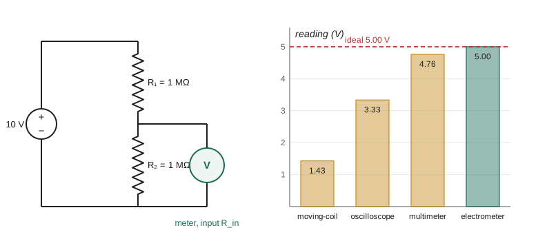
The same idea applies to current measurements, where an ammeter's own resistance, its burden, adds to the circuit and reduces the current it measures, and to every sensor: a thermometer exchanges heat with what it measures, a probe disturbs the field it samples. The general rule is to make the measuring device's influence small compared with the quantity measured, or to correct for it. The program below quantifies loading for a divider of two 1 MΩ resistors, whose true midpoint voltage is 5.000 V.

Alternating current and complex impedance

For sinusoidal signals, write voltages and currents as the real parts of complex exponentials, \(V(t) = \mathrm{Re}(\tilde{V}e^{i\omega t})\). Then resistors, capacitors and inductors all obey a generalized Ohm's law \(\tilde{V} = Z\tilde{I}\), with impedances

These follow from \(V = IR\), \(I = C\,dV/dt\) and \(V = L\,dI/dt\): differentiating \(e^{i\omega t}\) multiplies it by \(i\omega\). Impedances combine in series and parallel exactly like resistances, so the whole machinery of DC circuits carries over, with complex numbers. The magnitude \(|Z|\) gives the ratio of voltage and current amplitudes, and the phase of \(Z\) gives how far the voltage leads the current. A capacitor's impedance falls with frequency, so it blocks DC and passes high frequencies; an inductor does the opposite. At 1 kHz, a 100 nF capacitor has an impedance magnitude of 1.59 kΩ and a 100 mH inductor 628 Ω. In the program, a 1 kΩ resistor in series with the capacitor has \(|Z| = 1.88\) kΩ with the voltage lagging the current by 58 degrees.

The Wheatstone bridge

Many sensors produce a small change in a resistance: a platinum thermometer changes by 0.39 Ω per kelvin, a metal-foil strain gauge by about twice the strain times its resistance. Measuring a 0.1 parts in 1000 change in a resistance directly would require a meter of extraordinary accuracy. The Wheatstone bridge, popularized by Charles Wheatstone in 1843, avoids the problem by measuring a difference. Four resistors form two dividers fed from the same source; the output is the voltage between their midpoints. When the bridge is balanced, the output is zero whatever the supply voltage, and a small change \(\delta R\) in one arm produces an output

which can be amplified without the large steady voltage that would otherwise swamp it. The bridge is an example of a null method, comparing an unknown with a standard by adjusting for zero output. Null methods are powerful because the detector only needs to be sensitive, not calibrated.

import math, cmath
# 1. A voltage divider measured by meters of different input resistance.
Vs, R1, R2 = 10.0, 1.0e6, 1.0e6
ideal = Vs*R2/(R1 + R2)
for name, Rin in (("moving-coil meter, 20 kohm/V, 10 V range", 2.0e5), ("oscilloscope, 1 Mohm", 1.0e6), ("digital multimeter, 10 Mohm", 1.0e7), ("electrometer, 1e14 ohm", 1.0e14)):
    Rp = R2*Rin/(R2 + Rin)
    V = Vs*Rp/(R1 + Rp)
    print(f"{name:44s}: reads {V:6.3f} V (ideal {ideal:.3f} V, error {round((V/ideal - 1)*100, 1) + 0.0:+6.1f} parts per hundred)")
# 2. Complex impedances at 1 kHz.
f = 1000.0; w = 2*math.pi*f
R, C, Lh = 1000.0, 100e-9, 0.10
for name, Z in (("R + C in series", R + 1/(1j*w*C)), ("R + L in series", R + 1j*w*Lh), ("R parallel C", 1/(1/R + 1j*w*C))):
    print(f"{name:16s}: |Z| = {abs(Z):8.1f} ohm, phase = {math.degrees(cmath.phase(Z)):6.1f} degrees")
# 3. Wheatstone bridge: output for a small change in one arm (strain gauge, 120 ohm, gauge factor 2.0).
Vb, Rg = 5.0, 120.0
for strain in (1e-5, 1e-4, 1e-3):
    dR = Rg*2.0*strain
    Vout = Vb*((Rg + dR)/(2*Rg + dR) - 0.5)
    print(f"strain {strain:.0e}: bridge output {Vout*1e6:9.2f} microvolts (linear estimate {Vb*dR/(4*Rg)*1e6:9.2f})")

moving-coil meter, 20 kohm/V, 10 V range    : reads  1.429 V (ideal 5.000 V, error  -71.4 parts per hundred)
oscilloscope, 1 Mohm                        : reads  3.333 V (ideal 5.000 V, error  -33.3 parts per hundred)
digital multimeter, 10 Mohm                 : reads  4.762 V (ideal 5.000 V, error   -4.8 parts per hundred)
electrometer, 1e14 ohm                      : reads  5.000 V (ideal 5.000 V, error   +0.0 parts per hundred)
R + C in series : |Z| =   1879.6 ohm, phase =  -57.9 degrees
R + L in series : |Z| =   1181.0 ohm, phase =   32.1 degrees
R parallel C    : |Z| =    846.7 ohm, phase =  -32.1 degrees
strain 1e-05: bridge output     25.00 microvolts (linear estimate     25.00)
strain 1e-04: bridge output    249.98 microvolts (linear estimate    250.00)
strain 1e-03: bridge output   2497.50 microvolts (linear estimate   2500.00)

The moving-coil meter reads 1.43 V instead of 5.00 V, an error of 71 parts in 100, because its input resistance is comparable to the source resistance. The oscilloscope, at 1 MΩ, reads exactly a third low. Even the 10 MΩ multimeter is 5 parts in 100 low, which would be a serious systematic error in a precise experiment. Only the electrometer reads the true value. The bridge results show the linear approximation \(V_b\,\delta R/4R\) is excellent for small strains and still within 1 part in 1000 at a strain of \(10^{-3}\): a strain of \(10^{-5}\), a change in length of 10 μm per metre, produces 25 μV, easily measured after amplification.

Instruments of the bench

The digital multimeter measures DC and AC voltage, current and resistance. Its specifications deserve reading: accuracy is usually quoted as a fraction of reading plus a number of counts in the last digit, and AC ranges are accurate only within a stated frequency band. A true-rms meter computes the root mean square of any waveform; a cheaper average-responding meter assumes a sine wave and reads wrongly for other shapes. For resistance, a four-wire measurement passes current through one pair of leads and measures voltage with another, so that the resistance of the leads and contacts drops out; this is essential below about 10 Ω.

The oscilloscope displays voltage against time. Its essential specifications are bandwidth, the frequency at which a sine wave is displayed 3 dB low, and sampling rate. A 10:1 passive probe raises the input impedance to 10 MΩ and reduces capacitive loading, at the price of a tenfold attenuation; it must be compensated, by adjusting a small capacitor until a square calibration wave looks square, or it will distort fast edges. The trigger, which starts each sweep at the same point on a repeating signal, is the control most worth mastering. Signal generators supply sine, square and pulse waveforms and are the standard way to test a circuit's response; their output impedance, usually 50 Ω, forms a divider with the load like any source.

Calibration and traceability

An instrument's reading is only as good as its calibration. Every reputable meter is calibrated against a more accurate standard, which was calibrated against a better one, and so on up a chain that ends at a national metrology institute, the National Research Council of Canada, which realizes the SI units from their defining constants. This unbroken chain of comparisons, each with a stated uncertainty, is called traceability. For voltage, the top of the chain is the Josephson voltage standard, an array of superconducting junctions that produces voltages fixed by frequency and the ratio \(h/2e\); for resistance it is the quantum Hall effect, which gives resistances fixed by \(h/e^2\). Calibration drifts with time, temperature and use, so laboratory instruments carry calibration certificates with dates and are recalibrated on a schedule. In a research experiment, it is good practice to check an instrument against a known reference before and after a critical run: a standard resistor, a voltage reference chip, a known signal from a generator. If the check fails, you know the run is suspect; if you never checked, you will not know. The same logic applies to every sensor in the laboratory. A thermocouple should be checked at the ice point, a photodiode against a calibrated power meter, a balance with reference masses.

Grounding and interference

Many puzzling signals in the laboratory are interference. A loop of wire picks up the 60 Hz magnetic field of the building wiring, the frequency of the North American power grid, and its harmonics. Two instruments connected to ground at different points form a ground loop, in which a small current flows and appears as an offset or hum. Long cables act as antennas for radio-frequency noise. The remedies are standard: keep loops small, twist pairs of signal wires, use shielded coaxial cable with the shield grounded at one end, connect all grounds at a single point, and keep sensitive inputs away from transformers and motors. Lesson 6 shows how to reduce noise further by amplification and filtering, and lesson 7 by lock-in detection.