Separation of variables and the multipole expansion

The method of images works only for a few special geometries. A far more general technique for solving Laplace's equation is separation of variables, which looks for solutions that are products of functions of one coordinate each. Combined with the uniqueness theorem and the completeness of the resulting functions, it solves the square-pipe problem of lesson 7, the field around a sphere in a uniform field, and many others. In spherical coordinates the same method produces the Legendre polynomials, which lead to the multipole expansion: a systematic way of describing the potential of any localized charge distribution as seen from far away, as a sum of monopole, dipole, quadrupole and higher terms.

Separation in Cartesian coordinates

Take the long square pipe of lesson 7: \(0 \le x \le a\), \(0 \le y \le a\), with \(V = 0\) on three walls and \(V = V_0\) on the wall \(y = a\). Since nothing depends on \(z\), Laplace's equation is \(\partial^2 V/\partial x^2 + \partial^2 V/\partial y^2 = 0\). Look for solutions of the form \(V = X(x)\,Y(y)\). Substituting and dividing by \(XY\),

The first term depends only on \(x\) and the second only on \(y\). The only way their sum can vanish for all \(x\) and \(y\) is if each is a constant: \(X''/X = -k^2\) and \(Y''/Y = +k^2\). The sign is chosen because \(X\) must vanish at both \(x = 0\) and \(x = a\), which requires oscillating solutions, \(X = \sin(kx)\) with \(k = n\pi/a\) for \(n = 1, 2, 3, \dots\). Then \(Y\) must vanish at \(y = 0\), so \(Y = \sinh(n\pi y/a)\). Each product \(\sin(n\pi x/a)\sinh(n\pi y/a)\) satisfies Laplace's equation and the three grounded walls. None alone satisfies the condition on the top wall, but a sum of them can:

This is a Fourier sine series for the constant \(V_0\). Multiplying both sides by \(\sin(m\pi x/a)\) and integrating from 0 to \(a\), the orthogonality of the sines picks out one coefficient at a time: \(C_n\sinh(n\pi) = 4V_0/(n\pi)\) for odd \(n\) and zero for even \(n\). This is the series quoted in lesson 7, which agreed with relaxation to within the grid error. Joseph Fourier developed exactly this method for heat flow in 1807; the idea that any reasonable function can be expanded in sines is the completeness that makes separation of variables work.

Separation in spherical coordinates

For problems with azimuthal symmetry, where nothing depends on \(\phi\), Laplace's equation in spherical coordinates is

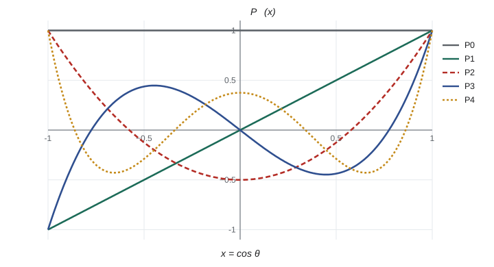
Trying \(V = R(r)\,\Theta(\theta)\) separates it into a radial equation, \(\frac{d}{dr}(r^2R') = l(l + 1)R\), with solutions \(r^l\) and \(r^{-(l+1)}\), and an angular equation, \(\frac{1}{\sin\theta}\frac{d}{d\theta}(\sin\theta\,\Theta') = -l(l + 1)\Theta\). The angular equation has solutions that are finite at both poles only when \(l\) is a non-negative integer, and then the solutions are the Legendre polynomials \(P_l(\cos\theta)\), studied by Adrien-Marie Legendre in the 1780s:

They satisfy Bonnet's recursion \((l + 1)P_{l+1} = (2l + 1)xP_l - lP_{l-1}\), which is how computers generate them, and they are orthogonal on \([-1, 1]\): \(\int_{-1}^{1}P_lP_{l'}\,dx = \frac{2}{2l + 1}\delta_{ll'}\). The general azimuthally symmetric solution is

A conducting sphere in a uniform field

Put a neutral conducting sphere of radius \(R\) into a uniform field \(\mathbf{E}_0 = E_0\hat{\mathbf{z}}\). Far away the potential must approach \(-E_0 z = -E_0 r\cos\theta\), and on the sphere it must be constant, which we may take as zero. The far-field condition allows only \(A_1 = -E_0\) among the \(A_l\). The condition on the sphere then requires \(B_1 = E_0R^3\) and all other \(B_l = 0\), giving

The induced charge is positive on the side the field points toward and negative on the other, and the second term in \(V\) is exactly the potential of a dipole at the centre. This is the result drawn in the conductor figure of lesson 6. Observe that the uniqueness theorem did the work: once the trial solution matched the boundary conditions, we knew it was right.

The multipole expansion

Now consider an arbitrary localized charge distribution, and ask for its potential far away. Using the law of cosines, \(1/\mathscr{r}\) can be expanded in powers of \(r'/r\), where \(r'\) is the distance of a source point from the origin and \(\alpha\) the angle between \(\mathbf{r}\) and \(\mathbf{r}'\):

and this is how the Legendre polynomials first entered physics: they are the coefficients in this generating function. Putting it into the potential integral,

The \(l = 0\) term is the monopole, \(Q/(4\pi\varepsilon_0 r)\), where \(Q\) is the total charge. The \(l = 1\) term is the dipole,

with \(\mathbf{p}\) the dipole moment. The \(l = 2\) term is the quadrupole, falling as \(1/r^3\), and so on. Far away, the lowest nonvanishing term dominates. A neutral molecule such as water is seen at large distances as a dipole; a neutral molecule with no dipole moment, such as carbon dioxide, is seen as a quadrupole. The dipole moment of a neutral distribution does not depend on the choice of origin, because shifting the origin by \(\mathbf{a}\) changes \(\mathbf{p}\) by \(-Q\mathbf{a}\), which vanishes when \(Q = 0\). For a charged distribution the dipole moment depends on the origin, and choosing the centre of charge makes it zero.

The dipole field follows from \(\mathbf{E} = -\nabla V_{\text{dip}}\). For \(\mathbf{p}\) along \(z\),

which falls off as \(1/r^3\): a dipole's field is weaker at large distance than a single charge's, because the two charges nearly cancel.

Legendre polynomials and a ring of charge

The program generates Legendre polynomials by recursion, checks their orthogonality numerically, and then uses them for a ring of radius 10 cm carrying 10 nC. On the axis of a ring every source point is at the same angle, and the expansion gives \(V = (kQ/r)\sum_l P_l(0)(a/r)^lP_l(\cos\theta)\) for \(r > a\); only even \(l\) contribute, because \(P_l(0)\) vanishes for odd \(l\). It compares the monopole term alone, the monopole plus quadrupole, and the series to \(l = 10\) with the exact potential computed by summing the ring. Finally it computes the dipole moment of a water-like molecule, with charge \(-0.8e\) on the oxygen and \(+0.4e\) on each hydrogen, about two different origins, and repeats the calculation for a charged ion.

import math
# 1. Legendre polynomials by Bonnet's recursion (l+1)P_{l+1} = (2l+1) x P_l - l P_{l-1}
def legendre(l, x):
    p0, p1 = 1.0, x
    if l == 0: return p0
    for n in range(1, l):
        p0, p1 = p1, ((2*n + 1)*x*p1 - n*p0)/(n + 1)
    return p1
print("x      P0      P1      P2      P3      P4")
for x in (-1.0, -0.5, 0.0, 0.5, 1.0):
    print(f"{x:4.1f} " + " ".join(f"{legendre(l, x)+0.0:7.4f}".replace("-0.0000", " 0.0000") for l in range(5)))
# orthogonality check: integral of P_l P_m from -1 to 1 equals 2/(2l+1) when l = m
N = 4000
for l, m in ((2, 2), (3, 3), (2, 4), (1, 3)):
    s = sum(legendre(l, -1 + 2*(i+.5)/N)*legendre(m, -1 + 2*(i+.5)/N)*2/N for i in range(N))
    print(f"integral P{l} P{m} = {(0.0 if abs(s) < 1e-5 else s):.5f}" + (f"   (2/(2l+1) = {2/(2*l+1):.5f})" if l == m else ""))

# 2. Multipole expansion of a ring of charge (radius a, charge Q) in the xy plane.
#    Off the ring, V(r, theta) = (kQ/r) sum_l P_l(0) (a/r)^l P_l(cos theta) for r > a.
k, a, Q = 8.9875517923e9, 0.1, 10e-9
def V_exact(r, th, n=4000):
    x, z = r*math.sin(th), r*math.cos(th)
    return sum(k*Q/n/math.sqrt((x - a*math.cos(2*math.pi*(i+.5)/n))**2
               + (a*math.sin(2*math.pi*(i+.5)/n))**2 + z*z) for i in range(n))
def V_multi(r, th, lmax):
    return k*Q/r*sum(legendre(l, 0.0)*(a/r)**l*legendre(l, math.cos(th)) for l in range(0, lmax + 1, 2))
for r, th in ((0.15, 0.0), (0.15, math.pi/2), (0.3, math.pi/3), (1.0, math.pi/4)):
    ex = V_exact(r, th)
    print(f"r = {r:4.2f}, theta = {math.degrees(th):4.1f} deg: exact {ex:8.3f} V | monopole {V_multi(r, th, 0):8.3f} "
          f"| +quadrupole {V_multi(r, th, 2):8.3f} | to l = 10 {V_multi(r, th, 10):8.3f}")

# 3. Dipole moment of a bent, water-like molecule (charges in units of e, positions in nm),
#    about two different origins; then the same for a charged ion, where the answer depends on the origin.
e, D = 1.602176634e-19, 3.33564e-30            # debye unit in C m
mol = [(-0.8, (0.0, 0.0)), (+0.4, (0.0757, 0.0586)), (+0.4, (-0.0757, 0.0586))]
ion = mol + [(+1.0, (0.0, -0.1))]
for name, qs in (("molecule", mol), ("ion", ion)):
    for o in ((0.0, 0.0), (0.5, 0.3)):
        px = sum(q*(r[0] - o[0]) for q, r in qs)*e*1e-9; py = sum(q*(r[1] - o[1]) for q, r in qs)*e*1e-9
        print(f"{name:8s} net charge {sum(q for q, _ in qs):+.1f} e, origin {o}: p = ({px/D:+.3f}, {py/D:+.3f}) D")

x      P0      P1      P2      P3      P4
-1.0  1.0000 -1.0000  1.0000 -1.0000  1.0000
-0.5  1.0000 -0.5000 -0.1250  0.4375 -0.2891
 0.0  1.0000  0.0000 -0.5000  0.0000  0.3750
 0.5  1.0000  0.5000 -0.1250 -0.4375 -0.2891
 1.0  1.0000  1.0000  1.0000  1.0000  1.0000
integral P2 P2 = 0.40000   (2/(2l+1) = 0.40000)
integral P3 P3 = 0.28571   (2/(2l+1) = 0.28571)
integral P2 P4 = 0.00000
integral P1 P3 = 0.00000
r = 0.15, theta =  0.0 deg: exact  498.540 V | monopole  599.170 | +quadrupole  466.021 | to l = 10  497.802
r = 0.15, theta = 90.0 deg: exact  690.286 V | monopole  599.170 | +quadrupole  665.745 | to l = 10  689.902
r = 0.30, theta = 60.0 deg: exact  301.222 V | monopole  299.585 | +quadrupole  301.666 | to l = 10  301.222
r = 1.00, theta = 45.0 deg: exact   89.762 V | monopole   89.876 | +quadrupole   89.763 | to l = 10   89.762
molecule net charge +0.0 e, origin (0.0, 0.0): p = (+0.000, +2.252) D
molecule net charge +0.0 e, origin (0.5, 0.3): p = (+0.000, +2.252) D
ion      net charge +1.0 e, origin (0.0, 0.0): p = (+0.000, -2.551) D
ion      net charge +1.0 e, origin (0.5, 0.3): p = (-24.016, -16.961) D

The orthogonality integrals come out as \(2/(2l + 1)\) on the diagonal and zero off it. For the ring, at 1.5 times its radius the monopole alone is off by 20% on the axis and 13% in the plane, with opposite signs: the ring's charge is spread in the plane, so the potential is larger there and smaller along the axis than a point charge would give. Adding the quadrupole term, which is negative along the axis and positive in the plane, corrects most of the error, and the series to \(l = 10\) is within 0.15%. At ten radii the monopole is already within 0.13%. The water-like molecule has a dipole moment of 2.25 debye whatever the origin; the real molecule's measured moment is 1.85 debye, because real charge distributions are not point charges. The ion's dipole moment changes completely when the origin moves, as the general argument predicts.