Laplace's equation, uniqueness and the method of images

Most real electrostatics problems do not hand us the charge distribution. Instead they specify conductors held at given potentials, or carrying given total charges, and ask for the field. The charge on the conductors is part of the answer, not the data. The way forward is to solve Laplace's equation, \(\nabla^2 V = 0\), in the region between the conductors, subject to boundary conditions on their surfaces. This lesson studies the properties of solutions of Laplace's equation, proves the uniqueness theorems that guarantee a solution is the solution, and introduces two powerful techniques: the method of images, which guesses the answer, and relaxation, which computes it numerically.

Properties of harmonic functions

Solutions of Laplace's equation are called harmonic functions. In one dimension Laplace's equation is \(d^2V/dx^2 = 0\), whose solutions are straight lines, \(V = mx + b\). Two properties of these simple solutions generalize to any number of dimensions. First, \(V(x)\) is the average of \(V(x + a)\) and \(V(x - a)\). Second, \(V\) has no local maxima or minima; its extreme values occur at the ends.

In three dimensions the corresponding statements are the mean value property and the maximum principle. If \(\nabla^2 V = 0\) in a region, then the value of \(V\) at any point equals the average of \(V\) over any sphere centred on that point and lying within the region,

To prove it for a single point charge \(q\) outside the sphere, compute the average of \(q/(4\pi\varepsilon_0\mathscr{r})\) over the sphere directly: the integral gives exactly the potential at the centre. Superposition extends the result to any collection of charges outside the sphere, which is to say to any harmonic function. An immediate consequence is the maximum principle: a harmonic function can have no local maximum or minimum inside the region, because then it could not equal its average over a small sphere around that point. Its extreme values lie on the boundary. Physically, this is Earnshaw's theorem, proved by Samuel Earnshaw in 1842: no arrangement of static charges can hold a charged particle in stable equilibrium, because the potential energy \(qV\) has no minimum in empty space. Ion traps get around the theorem with oscillating fields, and magnetic levitation of superconductors and diamagnets gets around it in other ways.

Uniqueness theorems

How do we know that a solution we have found is the only one? The first uniqueness theorem states that the solution of Laplace's equation in a volume is uniquely determined if \(V\) is specified on the boundary surface. Suppose \(V_1\) and \(V_2\) both satisfy Laplace's equation and the same boundary values. Their difference \(V_3 = V_1 - V_2\) satisfies Laplace's equation and is zero on the boundary. By the maximum principle, its largest and smallest values both lie on the boundary, where it is zero, so \(V_3 = 0\) everywhere. The same argument works for Poisson's equation with a given charge density inside, since the difference of two solutions is still harmonic.

A second uniqueness theorem covers conductors whose charges, rather than potentials, are given. In a volume surrounded by conductors and containing a specified charge density, the field is uniquely determined if the total charge on each conductor is given. The proof uses the identity \(\nabla\cdot(V_3\nabla V_3) = (\nabla V_3)^2 + V_3\nabla^2 V_3\) and the divergence theorem to show that the difference field \(\mathbf{E}_3 = \mathbf{E}_1 - \mathbf{E}_2\) has \(\int E_3^2\,d\tau = 0\), so it vanishes. The practical message of both theorems is liberating: if you can find a solution by any means, including inspired guessing, and it satisfies the equation and the boundary conditions, it is correct.

The method of images

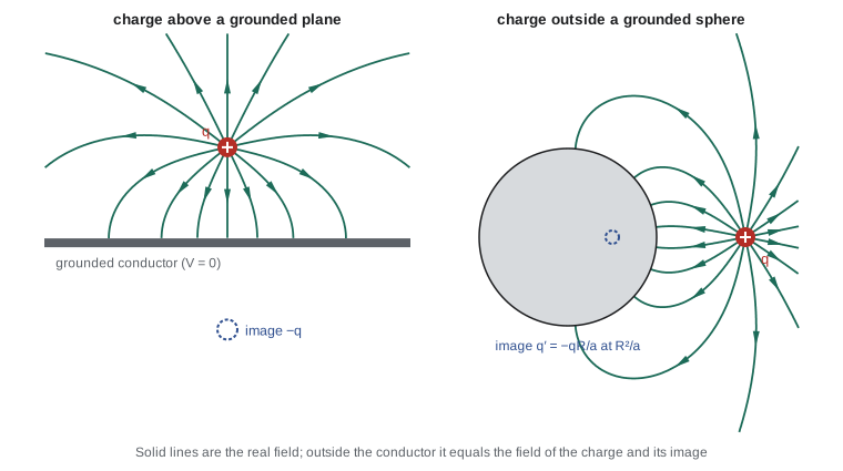
The classic example of inspired guessing is the method of images, introduced by William Thomson, later Lord Kelvin, in 1848. Place a point charge \(q\) at height \(d\) above an infinite grounded conducting plane. We want the potential in the region above the plane. The boundary conditions are \(V = 0\) on the plane and \(V \to 0\) far away. Now forget the conductor and consider instead a different problem: the charge \(q\) at \((0, 0, d)\) and an image charge \(-q\) at \((0, 0, -d)\). Its potential,

is zero on the plane \(z = 0\), goes to zero far away, and satisfies Poisson's equation with the single charge \(q\) in the region \(z > 0\). By the first uniqueness theorem, it is the solution of the original problem in that region. Below the plane the true potential is zero; the image is a fiction that reproduces the field only where we need it. From the potential we read off the induced surface charge, \(\sigma = -\varepsilon_0\,\partial V/\partial z\) at \(z = 0\),

which is negative, largest directly below the charge, and integrates to exactly \(-q\). The charge is attracted toward the plane by a force \(q^2/(4\pi\varepsilon_0(2d)^2)\), the force from its image.

The same idea works for a sphere. A point charge \(q\) at distance \(a\) from the centre of a grounded conducting sphere of radius \(R\) induces a charge distribution whose external field is that of an image charge \(q' = -qR/a\) placed at distance \(b = R^2/a\) from the centre, on the line toward \(q\). One can check directly that the potential of \(q\) and \(q'\) together vanishes at every point of the sphere. Images also solve problems with a charge between two intersecting grounded planes at certain angles, and a line charge near a conducting cylinder.

A boundary-value problem solved two ways

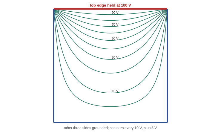
Not every problem has a neat image solution. Consider a long square pipe whose cross-section is the unit square, with three walls grounded and the top wall held at \(V_0 = 100\) V. The potential depends only on \(x\) and \(y\). Lesson 8 will solve this by separation of variables, finding

Here we preview it and solve the same problem numerically. Relaxation is based on the mean value property: on a grid with spacing \(h\), the discrete version of Laplace's equation says that the value at each interior point is the average of its four neighbours. Start with any guess, repeatedly replace each value by the average of its neighbours, and the grid relaxes toward the solution. Plain averaging, the Jacobi or Gauss–Seidel method, converges slowly. Successive over-relaxation overshoots each update by a factor \(\omega\) between 1 and 2, which speeds convergence dramatically; for a square grid of \(n\) points the optimal value is \(2/(1 + \sin(\pi/(n - 1)))\).

The program solves the square pipe on a 41 by 41 grid and compares the results with the series at four points. It then checks the image solution for the plane: it integrates the induced surface charge density over the plane, out to 400 times the height of the charge, and integrates the vertical force that charge exerts on \(q\), comparing with the image formula.

import math
# 1. Laplace's equation in a square box: three sides grounded, the top held at V0 = 100 V.
#    Solve by successive over-relaxation and compare with the separation-of-variables series.
n, V0 = 41, 100.0
V = [[0.0]*n for _ in range(n)]
for i in range(n): V[n-1][i] = V0            # row n-1 is the top edge y = 1
V[n-1][0] = V[n-1][n-1] = 50.0               # corners: average of the two edges
w = 2/(1 + math.sin(math.pi/(n - 1)))        # optimal over-relaxation factor
for sweep in range(1, 2001):
    change = 0.0
    for j in range(1, n-1):
        for i in range(1, n-1):
            new = 0.25*(V[j][i+1] + V[j][i-1] + V[j+1][i] + V[j-1][i])
            d = w*(new - V[j][i]); V[j][i] += d; change = max(change, abs(d))
    if change < 1e-7: break
print(f"SOR converged in {sweep} sweeps (omega = {w:.3f})")
def series(x, y, terms=200):
    # sinh(m pi y)/sinh(m pi) written as exp(m pi (y-1)) (1 - e^(-2 m pi y))/(1 - e^(-2 m pi)) to avoid overflow
    return sum(4*V0/(m*math.pi)*math.sin(m*math.pi*x)*math.exp(m*math.pi*(y - 1))
               *(1 - math.exp(-2*m*math.pi*y))/(1 - math.exp(-2*m*math.pi)) for m in range(1, 2*terms, 2))
for (x, y) in ((0.5, 0.5), (0.5, 0.25), (0.25, 0.75), (0.5, 0.9)):
    i, j = round(x*(n-1)), round(y*(n-1))
    print(f"  ({x:.2f}, {y:.2f}): relaxation {V[j][i]:7.3f} V, series {series(x, y):7.3f} V")

# 2. Point charge q a height d above a grounded plane: integrate the induced surface charge
#    sigma = -q d / (2 pi (r^2 + d^2)^(3/2)) and its pull on q, compare with the image force.
k = 8.9875517923e9; q, d = 1e-9, 0.02
Qind = 0.0; Fz = 0.0; N = 200000; Rmax = 400*d
for i in range(N):
    r = Rmax*((i + .5)/N)**2; dr = Rmax*2*(i + .5)/N**2   # finer rings near the axis
    sig = -q*d/(2*math.pi*(r*r + d*d)**1.5)
    dq = sig*2*math.pi*r*dr
    Qind += dq
    Fz += k*q*dq*d/(r*r + d*d)**1.5      # z component of the force on q (negative = toward plane)
print(f"induced charge = {Qind/q:.4f} q")
print(f"force on q from the surface charge {Fz*1e6:.3f} uN, image formula {-k*q*q/(2*d)**2*1e6:.3f} uN")

SOR converged in 161 sweeps (omega = 1.854)
  (0.50, 0.50): relaxation  25.000 V, series  25.000 V
  (0.50, 0.25): relaxation   9.545 V, series   9.541 V
  (0.25, 0.75): relaxation  43.199 V, series  43.203 V
  (0.50, 0.90): relaxation  80.151 V, series  80.169 V
induced charge = -0.9975 q
force on q from the surface charge -5.617 uN, image formula -5.617 uN

Over-relaxation converges in 161 sweeps, where plain Gauss–Seidel would need thousands. At the centre the potential is exactly 25 V, which has a beautiful explanation: by superposing four copies of the problem, each with a different wall at 100 V, we get a pipe with all four walls at 100 V, whose potential is 100 V everywhere; by symmetry each copy contributes equally at the centre. Elsewhere the relaxation values agree with the series to within about 0.02 V, the discretization error of a grid with spacing 1/40. The integrated surface charge is \(-0.9975q\); the missing 0.25% lies beyond 400 heights from the charge, since the induced charge beyond a radius \(s\) amounts to \(q\,d/\sqrt{s^2 + d^2}\), about \(q\,d/s\). The force computed from the surface charge, \(-5.617\) μN, matches the image formula exactly.