Capstone: magnetic fields in matter and applications

The final lesson does for magnetism what lesson 9 did for electricity: it describes how matter responds to a magnetic field and how that response feeds back on the field. The story has the same shape, with magnetization in place of polarization, bound currents in place of bound charges, and the auxiliary field \(\mathbf{H}\) in place of \(\mathbf{D}\). But magnetic materials are far more varied than dielectrics. Some weakly oppose an applied field, some weakly follow it, and a few, the ferromagnets, respond so strongly and with so much memory that they power the electrical grid and store data. The lesson ends with three applications that tie the course together: transformer cores, the superconducting magnets of MRI scanners, and the expulsion of magnetic fields by superconductors.

Magnetization and bound currents

Every atom contains moving charges, electrons orbiting and spinning, which carry magnetic dipole moments. In most materials these moments point randomly and cancel, but an applied field can line them up partially, producing a magnetization \(\mathbf{M}\), the magnetic dipole moment per unit volume. Following the steps of lesson 9 with the dipole vector potential of lesson 11 in place of the electric dipole potential, the field of a magnetized object turns out to be exactly that of bound currents,

The picture is easy to see for a uniformly magnetized cylinder. Each atomic dipole is a tiny current loop. Inside, adjacent loops carry currents in opposite directions where they touch, and cancel. At the curved surface nothing cancels, and the loops add up to a surface current circling the cylinder, \(K_b = M\). A uniformly magnetized cylinder is magnetically identical to a solenoid with \(nI = M\). These are real currents, of electrons bound to atoms, and they produce real fields.

The auxiliary field H

Separating the current into free current, which we control by connecting wires, and bound current, Ampère's law reads \(\nabla\times\mathbf{B}/\mu_0 = \mathbf{J}_f + \nabla\times\mathbf{M}\). Collecting the curls defines

\(\mathbf{H}\) is useful because the free current is what an experimenter sets: the current in a coil determines \(\mathbf{H}\) directly in symmetric geometries, and \(\mathbf{B}\) then depends on the material. Like \(\mathbf{D}\), however, \(\mathbf{H}\) is not determined by the free current alone, because its divergence, \(-\nabla\cdot\mathbf{M}\), need not vanish. \(\mathbf{H}\) is measured in amperes per metre. Engineers often call \(\mathbf{H}\) the magnetic field and \(\mathbf{B}\) the magnetic flux density; physicists usually reserve the name field for \(\mathbf{B}\). In linear materials \(\mathbf{M} = \chi_m\mathbf{H}\) and

Three kinds of magnetic response

Diamagnetic materials have small negative susceptibility, of order \(-10^{-5}\): an applied field induces atomic currents that oppose it, a consequence of Lenz's law at the atomic scale. Every material is diamagnetic, but the effect is usually masked by stronger ones. Water and living tissue are diamagnetic, and in the 1990s Andre Geim's group famously levitated a live frog in the 16-tesla field of a powerful magnet, since a strong enough field gradient lifts any diamagnetic object. Paramagnetic materials, such as aluminium and oxygen, contain atoms with permanent magnetic moments that partially align with the field, giving a small positive susceptibility of order \(10^{-5}\) to \(10^{-3}\) that falls with temperature as \(1/T\), Curie's law of 1895.

Ferromagnets, chiefly iron, nickel, cobalt and many of their alloys and compounds, are different in kind. A quantum-mechanical exchange interaction makes neighbouring atomic moments align spontaneously, forming domains, regions perhaps a micrometre to a millimetre across, each magnetized to saturation. In an unmagnetized piece the domains point in different directions and cancel. An applied field grows the favourably oriented domains at the expense of others, so the magnetization can reach saturation, more than \(10^6\) A/m in iron, in modest fields. Above the Curie temperature, 1043 K for iron, thermal agitation destroys the alignment and the material becomes paramagnetic. The response is strongly nonlinear and history dependent, so the susceptibility is not a constant at all.

Hysteresis

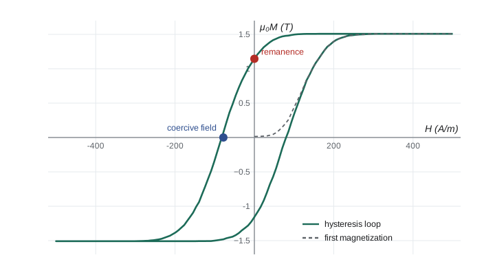
If you magnetize a ferromagnet to saturation and then reduce the applied field to zero, the magnetization does not return to zero. Some domain alignment remains, the remanence, which is what makes a permanent magnet. To remove it you must apply a reverse field, the coercive field. Cycling the field back and forth traces a closed loop in the B–H plane, the hysteresis loop, a name coined by James Alfred Ewing in 1881. The area of the loop equals the energy dissipated as heat per unit volume per cycle, \(\oint H\,dB\). Materials for transformer cores need a small loop, which means low coercivity, so that little energy is lost each cycle; materials for permanent magnets need a large one, with high remanence and high coercivity, so that they keep their magnetization.

The Preisach model of 1935 captures hysteresis with a simple picture. Imagine the material as a large number of tiny elements, each of which switches its magnetization up when the applied field exceeds its own upper threshold and down when the field falls below its lower threshold. Different elements have different thresholds, so as the field rises, more and more switch up, and as it falls they switch down at lower fields. The program uses 4000 such elements, with thresholds spread randomly, demagnetizes the sample by an alternating field of decreasing size, then traces the first magnetization curve and a full loop.

Applications

A transformer core exploits the large permeability of soft iron. With \(\mu_r\) in the thousands, a modest current in the primary coil produces a field of order a tesla in the core, and nearly all the flux stays inside the iron, linking the secondary coil. The cost is the hysteresis loss each cycle, along with eddy currents in the iron, which is why cores are made of thin laminated sheets of silicon steel with a narrow loop. In North America the grid runs at 60 Hz, so a core goes round its loop 60 times a second.

A magnetic resonance imaging scanner needs a large, extremely uniform and stable field, typically 1.5 or 3 teslas, over a region big enough for a person. Iron saturates near 2 T, so the field must come from current alone, and the currents needed are large: \(nI\) of over a million ampere-turns per metre. Resistive wire would dissipate megawatts. Instead the coils are wound from niobium–titanium superconductor, cooled by liquid helium to about 4 K, where it carries current with no resistance at all. Once energized, the magnet runs in persistent mode, with the current circulating indefinitely, and the field drifts by only parts per million over months. Correction coils, like an elaborate version of the Helmholtz pair of lesson 10, make the field uniform to a few parts per million over the imaging volume.

Superconductors do more than conduct without loss. Heike Kamerlingh Onnes discovered superconductivity in mercury at 4.2 K in 1911, and in 1933 Walther Meissner and Robert Ochsenfeld found that a superconductor expels magnetic field from its interior when cooled through its transition. This Meissner effect makes a superconductor a perfect diamagnet, \(\chi_m = -1\). The field does penetrate a short distance, decaying exponentially over the London penetration depth, typically tens to hundreds of nanometres, as Fritz and Heinz London explained in 1935. Expulsion of field is why a small magnet levitates stably above a cooled superconductor, a striking exception to the spirit of Earnshaw's theorem made possible because the superconductor is not a static charge distribution.

import math, random
mu0 = 4e-7*math.pi
rnd = random.Random(381)
# 1. A Preisach model of hysteresis: many tiny magnetic switches ("hysterons"), each flipping up
#    when H rises above its own a and down when H falls below its own b (a > b).
N = 4000
hyst = []
for _ in range(N):
    c = rnd.gauss(0.0, 60.0); w = abs(rnd.gauss(80.0, 30.0))    # A/m: bias and half-width
    hyst.append([c + w, c - w, -1])                                # up threshold, down threshold, state
Ms = 1.2e6                                                         # A/m, saturation magnetization (steel-like)
def M_of(H):
    for h in hyst:
        if H >= h[0]: h[2] = 1
        elif H <= h[1]: h[2] = -1
    return Ms*sum(h[2] for h in hyst)/N
for k in range(60): M_of(500.0*(1 - k/60)*(-1)**k)        # demagnetize with a shrinking alternating field
M_of(0.0)
Hmax, steps = 500.0, 400
path = [Hmax*math.sin(2*math.pi*i/steps) for i in range(steps + 1)]
for H in path[: steps//4 + 1]: M_of(H)              # first rise from the demagnetized state
loop = [(H, M_of(H)) for H in path[steps//4:] + path[1: steps//4 + 1]]
Br = max(mu0*M for H, M in loop if abs(H) < 1.3 and M > 0)
Hc = min(abs(H) for H, M in loop if abs(M) < 0.02*Ms)
area = sum(mu0*(loop[i][1] + loop[i+1][1])/2*(loop[i+1][0] - loop[i][0]) for i in range(len(loop) - 1))
print(f"remanent field B_r about {Br:.2f} T, coercive field H_c about {Hc:.0f} A/m")
print(f"loss per cycle = area of the B-H loop: {abs(area):.1f} J/m^3; at 60 Hz in 0.01 m^3 of core: {abs(area)*60*0.01:.0f} W")

# 2. MRI magnet: a superconducting solenoid producing 1.5 T and 3 T
for B in (1.5, 3.0):
    nI = B/mu0
    print(f"{B} T needs n I = {nI:.3e} A-turns per m; with 400 A that is {nI/400:.0f} turns per m; "
          f"field energy density {B*B/(2*mu0)/1e6:.2f} MJ/m^3")

# 3. Transformer core: an iron core (relative permeability 4000) multiplies the field of a coil
mur, n, I = 4000, 500, 0.5
H = n*I
print(f"core: H = {H:.0f} A/m, B with core {mu0*mur*H:.3f} T, without {mu0*H*1e3:.3f} mT")

# 4. Superconductor: London penetration depth and the Meissner screening of a 0.1 T field
lam = 50e-9
for x in (0, 50e-9, 100e-9, 250e-9):
    print(f"depth {x*1e9:5.0f} nm: B = {0.1*math.exp(-x/lam)*1e3:7.3f} mT")

remanent field B_r about 1.15 T, coercive field H_c about 78 A/m
loss per cycle = area of the B-H loop: 489.2 J/m^3; at 60 Hz in 0.01 m^3 of core: 294 W
1.5 T needs n I = 1.194e+06 A-turns per m; with 400 A that is 2984 turns per m; field energy density 0.90 MJ/m^3
3.0 T needs n I = 2.387e+06 A-turns per m; with 400 A that is 5968 turns per m; field energy density 3.58 MJ/m^3
core: H = 250 A/m, B with core 1.257 T, without 0.314 mT
depth     0 nm: B = 100.000 mT
depth    50 nm: B =  36.788 mT
depth   100 nm: B =  13.534 mT
depth   250 nm: B =   0.674 mT

The Preisach model produces a loop with a remanent field of about 1.1 T and a coercive field of about 80 A/m, values typical of a soft steel. The loop area, about 490 J/m\(^3\) per cycle, means that a core of one hundredth of a cubic metre, about 80 kg of steel, dissipates roughly 300 W at 60 Hz from hysteresis alone; grain-oriented transformer steel does several times better. The MRI calculation shows that a 1.5 T magnet with 400 A in its superconducting wire needs about 3000 turns per metre, and stores 0.9 MJ in every cubic metre of field, so that quenching, the sudden loss of superconductivity, must be managed carefully to dump that energy safely. The transformer core multiplies the field of a 500-turn coil carrying half an ampere from 0.3 mT to 1.26 T, a factor of 4000. Finally, a 0.1 T field falls to under 1% of its surface value within 250 nm of the surface of a superconductor with a 50 nm penetration depth.

Looking back and ahead

This course started from Coulomb's and the Biot–Savart laws and ended with four equations: \(\nabla\cdot\mathbf{D} = \rho_f\), \(\nabla\times\mathbf{E} = \mathbf{0}\), \(\nabla\cdot\mathbf{B} = 0\) and \(\nabla\times\mathbf{H} = \mathbf{J}_f\), together with the constitutive relations of matter. Along the way it developed potentials, boundary conditions, images, separation of variables, multipoles, relaxation and the physics of dielectrics and magnets. PHYS-382 removes the restriction to static fields. Faraday's law adds \(-\partial\mathbf{B}/\partial t\) to the curl of \(\mathbf{E}\), Maxwell's displacement current adds \(\partial\mathbf{D}/\partial t\) to the curl of \(\mathbf{H}\), and the resulting equations predict electromagnetic waves travelling at \(1/\sqrt{\varepsilon_0\mu_0}\), the number computed in lesson 1.