Curvilinear coordinates and the Dirac delta function

Most field problems with any symmetry are easier in spherical or cylindrical coordinates than in Cartesian ones. A point charge, a charged sphere and an atom have spherical symmetry; a wire, a coaxial cable and a solenoid have cylindrical symmetry. This lesson develops the vector operators in those coordinates and then confronts a puzzle that sits at the heart of electrostatics: the field of a point charge appears to have zero divergence everywhere, yet Gauss's law says its flux through a surrounding sphere is not zero. The resolution is the Dirac delta function, a mathematical object that lets point charges, line charges and surface charges be written as densities and placed inside differential equations.

Spherical coordinates

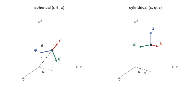
A point is located by its distance \(r\) from the origin, the polar angle \(\theta\) measured down from the z axis, and the azimuthal angle \(\phi\) measured around the z axis from the x axis:

At every point there are three mutually perpendicular unit vectors: \(\hat{\mathbf{r}}\) points away from the origin, \(\hat{\boldsymbol{\theta}}\) points in the direction of increasing \(\theta\) (southward on a globe), and \(\hat{\boldsymbol{\phi}}\) points in the direction of increasing \(\phi\) (eastward). Unlike \(\hat{\mathbf{x}}\), \(\hat{\mathbf{y}}\), \(\hat{\mathbf{z}}\), these unit vectors change direction from point to point. That is the source of nearly every error made with curvilinear coordinates: you may not pull \(\hat{\mathbf{r}}\) out of an integral over angles, because it points in different directions at different places. When integrating a vector, convert to Cartesian components first.

An infinitesimal displacement has components \(dr\), \(r\,d\theta\) and \(r\sin\theta\,d\phi\), so the line, area and volume elements are

Because the steps in \(\theta\) and \(\phi\) are not lengths, the vector operators acquire scale factors. The gradient, divergence, curl and Laplacian are

The curl has a similar structure and is listed in the formula sheet of every electromagnetism text. You do not need to memorize these, but you must recognize where the factors come from: each derivative with respect to an angle is divided by the corresponding scale factor, \(r\) or \(r\sin\theta\), and in the divergence each component is first multiplied by the area of the face it crosses.

Cylindrical coordinates

Cylindrical coordinates use the perpendicular distance \(s\) from the z axis, the azimuthal angle \(\phi\), and \(z\):

Many books write \(r\) or \(\rho\) for the cylindrical radius; we use \(s\) to avoid confusion with the spherical \(r\) and with charge density \(\rho\). The divergence and Laplacian are

A paradox about the point charge

Consider the field \(\mathbf{v} = \hat{\mathbf{r}}/r^2\), which is the field of a point charge up to a constant. Its divergence, from the spherical formula, is

But the flux through a sphere of radius \(R\) is \(\oint (1/R^2)\,R^2\sin\theta\,d\theta\,d\phi = 4\pi\), independent of \(R\). The divergence theorem seems to fail: the volume integral of zero is zero, but the surface integral is \(4\pi\). The flaw is at the origin, where \(\mathbf{v}\) blows up and the formula for the divergence is meaningless. All of the divergence is concentrated at that single point, and its integral over any volume containing the origin is \(4\pi\). No ordinary function behaves like this. We need a new kind of object.

The Dirac delta function

In one dimension, the Dirac delta function \(\delta(x)\) is defined by two properties: it is zero for every \(x \ne 0\), and its integral over any interval containing zero is 1. It is best thought of as the limit of a sequence of ever taller, narrower spikes of unit area, for example Gaussians of width \(\varepsilon\),

Strictly, the delta function is not a function but a distribution, defined by what it does inside an integral. Its essential property follows directly: since \(\delta(x - a)\) is zero except at \(x = a\), a smooth function multiplying it may be replaced by its value there,

Paul Dirac introduced the notation in his quantum mechanics of the late 1920s, although similar objects had been used by Heaviside and others. In three dimensions, \(\delta^3(\mathbf{r}) = \delta(x)\,\delta(y)\,\delta(z)\), with \(\int \delta^3(\mathbf{r})\,d\tau = 1\) over any volume containing the origin. The resolution of the paradox is then

and since \(\hat{\mathbf{r}}/r^2 = -\nabla(1/r)\), the Laplacian of \(1/r\) is \(-4\pi\delta^3(\mathbf{r})\). This single identity is the mathematical core of electrostatics. A point charge \(q\) at \(\mathbf{r}'\) can now be written as a charge density \(\rho(\mathbf{r}) = q\,\delta^3(\mathbf{r} - \mathbf{r}')\), and Gauss's law in differential form, \(\nabla\cdot\mathbf{E} = \rho/\varepsilon_0\), holds for point charges as well as smooth distributions.

Two further rules are used constantly. Scaling the argument rescales the spike: \(\delta(kx) = \delta(x)/|k|\), as substitution in the defining integral shows. And a surface charge \(\sigma\) on the plane \(z = 0\) is the volume density \(\rho = \sigma\,\delta(z)\); a line charge \(\lambda\) along the z axis is \(\rho = \lambda\,\delta(x)\,\delta(y)\). With these, every kind of charge distribution, from points to smooth clouds, can be handled by the same formulas.

Why divergence and curl are enough

The delta function also answers a question that underlies the whole course: if we know the divergence and the curl of a vector field everywhere, do we know the field? The Helmholtz theorem, due to Hermann von Helmholtz in the 1850s, says yes, provided the field falls to zero at infinity faster than \(1/r\). Given \(\nabla\cdot\mathbf{F} = D\) and \(\nabla\times\mathbf{F} = \mathbf{C}\), with \(\nabla\cdot\mathbf{C} = 0\) as consistency requires, the field is

The proof uses exactly the identity \(\nabla^2(1/\mathscr{r}) = -4\pi\delta^3(\mathbf{r} - \mathbf{r}')\): taking the divergence of the first term returns \(D\), and taking the curl of the second returns \(\mathbf{C}\). Uniqueness follows because the difference of two solutions would have zero divergence and zero curl everywhere, so it would be the gradient of a function obeying Laplace's equation, and such a function that vanishes at infinity is zero. The theorem explains why Maxwell's equations are stated as divergence and curl equations: together with a condition at infinity, they say everything there is to say about the fields. In electrostatics the curl is zero, so only the first term survives, and the integral inside it is the electric potential of lesson 5. In magnetostatics the divergence is zero, so only the second term survives, and its integral is the vector potential of lesson 11.

It is worth seeing how the delta function makes a line charge fit the same formulas. A uniform line charge \(\lambda\) along the z axis has volume density \(\rho = \lambda\,\delta(x)\,\delta(y)\). Integrating over a slab of thickness \(dz\) that crosses the axis gives \(\lambda\,dz\), as it should. In cylindrical coordinates the same density is \(\rho = \lambda\,\delta(s)/(2\pi s)\), where the factor \(1/(2\pi s)\) compensates for the volume element \(s\,ds\,d\phi\,dz\). Such conversions between coordinate systems are a frequent source of errors, and the safe test is always to integrate the density and confirm that it returns the right total charge.

Checking the delta function numerically

The program performs three checks. First it computes the flux of \(\hat{\mathbf{r}}/r^2\) through spheres of different radii and centres, by summing over a grid of surface patches. Second it integrates a test function \(f(x) = \cos x + x^3\) against Gaussians of decreasing width, which should approach \(f(0) = 1\). Third it computes the gradient of \(V = r^2\cos\theta\) from the spherical formula and compares it with a Cartesian finite-difference gradient resolved onto \(\hat{\mathbf{r}}\) and \(\hat{\boldsymbol{\theta}}\).

import math
# 1. The field r_hat/r^2 has zero divergence away from the origin, yet its flux through
#    any sphere around the origin is 4 pi: the divergence is 4 pi delta^3(r).
def flux_sphere(R, n=200, center=(0, 0, 0)):
    tot = 0.0
    for i in range(n):
        th = math.pi*(i + .5)/n
        for j in range(2*n):
            ph = 2*math.pi*(j + .5)/(2*n)
            nx, ny, nz = math.sin(th)*math.cos(ph), math.sin(th)*math.sin(ph), math.cos(th)
            x, y, z = center[0] + R*nx, center[1] + R*ny, center[2] + R*nz
            r = math.sqrt(x*x + y*y + z*z)
            Fn = (x*nx + y*ny + z*nz) / r**3
            tot += Fn * R*R*math.sin(th) * (math.pi/n) * (math.pi/n)
    return tot
for R, c in ((0.5, (0, 0, 0)), (3.0, (0, 0, 0)), (1.0, (0.4, 0.2, 0.0)), (1.0, (2.0, 0.0, 0.0))):
    print(f"sphere R={R} at {c}: flux/(4 pi) = {flux_sphere(R, center=c)/(4*math.pi):.4f}")

# 2. A sequence of Gaussians tends to the Dirac delta: integral of g_eps(x) f(x) -> f(0)
f = lambda x: math.cos(x) + x**3
for eps in (1.0, 0.3, 0.1, 0.03):
    N, L = 20000, 10*eps
    s = sum(math.exp(-((-L + 2*L*(i+.5)/N)/eps)**2/2)/(eps*math.sqrt(2*math.pi))
            * f(-L + 2*L*(i+.5)/N) * 2*L/N for i in range(N))
    print(f"eps = {eps:5.2f}: integral = {s:.6f}   (f(0) = 1)")

# 3. Gradient in spherical coordinates: V = r^2 cos(theta), checked against Cartesian
r, th = 1.5, 0.7
Er = 2*r*math.cos(th); Eth = (1/r)*(-r*r*math.sin(th))
x, z = r*math.sin(th), r*math.cos(th)          # V = z*sqrt(x^2+z^2) in the xz plane
h = 1e-6
V = lambda x, z: z*math.sqrt(x*x + z*z)
gx = (V(x+h, z) - V(x-h, z))/(2*h); gz = (V(x, z+h) - V(x, z-h))/(2*h)
print(f"spherical (dV/dr, (1/r)dV/dth) = ({Er:.5f}, {Eth:.5f}); "
      f"from Cartesian = ({gx*math.sin(th)+gz*math.cos(th):.5f}, {gx*math.cos(th)-gz*math.sin(th):.5f})")

sphere R=0.5 at (0, 0, 0): flux/(4 pi) = 1.0000
sphere R=3.0 at (0, 0, 0): flux/(4 pi) = 1.0000
sphere R=1.0 at (0.4, 0.2, 0.0): flux/(4 pi) = 1.0000
sphere R=1.0 at (2.0, 0.0, 0.0): flux/(4 pi) = 0.0000
eps =  1.00: integral = 0.606531   (f(0) = 1)
eps =  0.30: integral = 0.955997   (f(0) = 1)
eps =  0.10: integral = 0.995012   (f(0) = 1)
eps =  0.03: integral = 0.999550   (f(0) = 1)
spherical (dV/dr, (1/r)dV/dth) = (2.29453, -0.96633); from Cartesian = (2.29453, -0.96633)

Every sphere that encloses the origin, large, small or shifted to one side, has flux exactly \(4\pi\); the sphere centred at (2, 0, 0) with radius 1, which does not enclose the origin, has flux zero. This is the delta function at work: all of the divergence sits at one point, and the flux counts whether that point is inside. The Gaussian integrals approach \(f(0) = 1\) as the width shrinks, and the error falls as \(\varepsilon^2\), because the first correction is proportional to \(f''(0)\varepsilon^2/2 = -\varepsilon^2/2\): for \(\varepsilon = 0.1\) the integral is 0.99501, close to \(1 - 0.005\). The spherical gradient formula agrees with the Cartesian one to five decimal places, which is a useful habit to adopt whenever you are unsure of a curvilinear formula.