The Boltzmann distribution, equipartition and the Maxwell speed distribution

Counting microstates of an isolated system, as in lesson 10, is clean but awkward: most systems we care about are not isolated but sit in contact with surroundings at a fixed temperature. A molecule in a gas exchanges energy with all the others; an atom in a crystal exchanges energy with the rest of the lattice. This lesson derives the probability that such a system is found in a state of given energy, the Boltzmann distribution, which is the single most useful result of statistical mechanics. From it follow the partition function, the equipartition theorem, the Maxwell speed distribution of lesson 4, the heat capacities of lesson 5, the barometric formula for the atmosphere and the slow leakage of light gases into space.

The Boltzmann factor

Consider a small system, such as a single atom or molecule, in thermal contact with a large reservoir at temperature \(T\). The combined system is isolated with total energy \(U_0\), so by the fundamental assumption all its microstates are equally likely. Pick one particular microstate \(s\) of the small system, with energy \(E_s\). The reservoir then has energy \(U_0 - E_s\), and the number of ways it can arrange itself is \(\Omega_R(U_0 - E_s)\). The probability of finding the small system in state \(s\) is proportional to that number. Because \(E_s\) is tiny compared with \(U_0\), expand the reservoir's entropy:

Exponentiating gives \(\Omega_R \propto e^{-E_s/kT}\), so

The factor \(e^{-E_s/kT}\) is the Boltzmann factor, and the normalizing sum \(Z\) is the partition function, from the German Zustandssumme, sum over states. The derivation used nothing about the small system except that it is small: the result holds for an atom, a molecule, a spin, a vibrational mode or any subsystem in contact with a large environment. Note that it gives the probability of a single microstate. The probability of an energy level is the Boltzmann factor times the number of states with that energy, its degeneracy. High-energy states are individually unlikely, but there may be many of them.

It is convenient to write \(\beta = 1/kT\). The partition function then encodes all the thermodynamics. The mean energy is

and the Helmholtz free energy is \(F = -kT\ln Z\), from which pressure, entropy and heat capacity follow by differentiation. For \(N\) independent distinguishable subsystems, partition functions multiply; for \(N\) identical, indistinguishable gas molecules, \(Z_N = Z_1^N/N!\), the same factor that appeared in the Sackur–Tetrode counting.

The two-level system

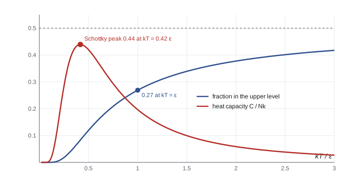
The simplest example has two states, with energies 0 and \(\varepsilon\): a magnetic moment in a field, pointing along or against it, or a molecule with one low-lying excited state. Then \(Z = 1 + e^{-\beta\varepsilon}\), the fraction in the upper state is \(e^{-\beta\varepsilon}/(1 + e^{-\beta\varepsilon})\), and the mean energy is \(\varepsilon/(e^{\beta\varepsilon} + 1)\). At low temperature almost everything is in the ground state; at high temperature the two states become equally populated, but never more than equally. The heat capacity,

vanishes at both extremes and has a peak, the Schottky anomaly, near \(kT = 0.42\varepsilon\). Such peaks in the low-temperature heat capacities of crystals reveal the presence of low-lying energy levels, for example of magnetic ions, and were explained by Walter Schottky in 1922.

If a spin system is prepared with more spins in the upper state than the lower, for example by suddenly reversing the magnetic field, the Boltzmann formula can describe it only with a negative temperature. Such states, first produced with nuclear spins in lithium fluoride by Edward Purcell and Robert Pound in 1951, are hotter than any positive temperature: when brought into contact with an ordinary system, they give energy to it. They exist only for systems with a maximum energy, and they reinforce the lesson that temperature is defined by \(\partial S/\partial U\), not by energy per particle.

The quantum oscillator

A harmonic oscillator with levels \(\hbar\omega(j + \frac12)\) has

Differentiating \(\langle E\rangle\) with respect to \(T\) gives exactly the Einstein heat capacity of lesson 5. At high temperature, \(e^{\beta\hbar\omega} - 1 \approx \beta\hbar\omega\) and \(\langle E\rangle \to kT\), the classical value; at low temperature the excitations die away exponentially. The term \(1/(e^{\beta\hbar\omega} - 1)\) is the mean number of quanta in the oscillator. Applied to the modes of the electromagnetic field in a cavity, where each mode is an oscillator and the quanta are photons, it gives Planck's radiation law of lesson 6.

Equipartition

In classical mechanics the sum over states becomes an integral over positions and momenta. Suppose the energy contains a term quadratic in some variable \(q\), \(E = cq^2 + (\text{terms not involving } q)\). The average of that term is

This is the equipartition theorem: in classical equilibrium, every quadratic degree of freedom has average energy \(\frac12 kT\), whatever its coefficient \(c\). Translation gives three such terms, \(\frac12 m(v_x^2 + v_y^2 + v_z^2)\); rotation of a diatomic molecule two more; a vibration two, one kinetic and one potential. The theorem justifies the heat capacities of lesson 5, and the quantum oscillator shows when it fails: a degree of freedom counts only if \(kT\) is large compared with its level spacing. Equipartition also explains thermal noise. The voltage fluctuations across a resistor, discovered by John Johnson and explained by Harry Nyquist in 1928, have mean square \(4kTR\,\Delta f\) in a bandwidth \(\Delta f\); measuring them is one of the ways the Boltzmann constant was determined for the 2019 redefinition of the kelvin.

The Maxwell distribution from Boltzmann

For a molecule in an ideal gas, the energy is \(\frac12 mv^2\) and the states are labelled by the velocity. The Boltzmann factor gives the probability density of a velocity vector as proportional to \(e^{-mv^2/2kT}\), which is the product of three independent Gaussians, exactly Maxwell's assumption. Counting velocity vectors in a shell of radius \(v\), whose volume is \(4\pi v^2\,dv\), gives Maxwell's speed distribution of lesson 4, now derived rather than assumed. The program samples velocities this way, with Gaussian random numbers generated by the Box–Muller method, and checks the characteristic speeds and equipartition.

Gravity, escape and activation

In a gravitational field, a molecule at height \(z\) has potential energy \(mgz\), so in an isothermal atmosphere the density falls as \(e^{-mgz/kT}\), the barometric formula, with scale height \(H = kT/(mg)\), about 7 to 8 km for air. Jean Perrin used the same law in 1908 to measure Avogadro's number from the heights of tiny resin spheres suspended in water, providing decisive evidence for the reality of atoms. The tail of the Maxwell distribution at the top of an atmosphere determines which gases a planet can keep: molecules faster than the escape speed, 10.8 km/s at Earth's exobase about 500 km up, can leave. The program shows why the Earth has lost its primordial hydrogen and helium but kept its oxygen and nitrogen. Finally, the Boltzmann factor explains why chemical reaction rates rise so steeply with temperature: if a reaction needs an activation energy \(E_a\), its rate is proportional to \(e^{-E_a/kT}\), the Arrhenius law, proposed by Svante Arrhenius in 1889.

import math, random
k = 1.380649e-23; u = 1.66053907e-27; eV = 1.602176634e-19

# 1. Two-level system: populations and the Schottky heat capacity (units: k, energy gap eps)
print(" kT/eps   upper fraction   C/(N k)")
for t in (0.1, 0.2, 0.42, 1.0, 2.0, 10.0):
    x = 1 / t
    p_up = math.exp(-x) / (1 + math.exp(-x))
    C = x * x * math.exp(x) / (1 + math.exp(x))**2
    print(f"  {t:5.2f}       {p_up:.4f}        {C:.4f}")

# 2. Characteristic speeds of nitrogen at 300 K, and a sample drawn by Box-Muller
m, T = 28.0 * u, 300.0
vp, vmean, vrms = math.sqrt(2 * k * T / m), math.sqrt(8 * k * T / (math.pi * m)), math.sqrt(3 * k * T / m)
print(f"\nN2 at 300 K: most probable {vp:.0f} m/s, mean {vmean:.0f} m/s, rms {vrms:.0f} m/s")
rnd = random.Random(261)
s = math.sqrt(k * T / m)
def gauss():
    u1, u2 = 1 - rnd.random(), rnd.random()
    return math.sqrt(-2 * math.log(u1)) * math.cos(2 * math.pi * u2)
sample = [math.sqrt(sum((s * gauss())**2 for _ in range(3))) for _ in range(60000)]
mean = sum(sample) / len(sample); rms = math.sqrt(sum(v * v for v in sample) / len(sample))
print(f"sample of 60000: mean {mean:.1f} m/s, rms {rms:.1f} m/s")
print(f"equipartition: <(1/2) m vx^2> / (kT/2) = {sum(0.5 * m * (s * gauss())**2 for _ in range(60000)) / 60000 / (0.5 * k * T):.4f}")

# 3. Isothermal atmosphere: scale height and pressure with altitude
g = 9.81
H = k * 250 / (29.0 * u * g)
print(f"\nscale height of an isothermal 250 K atmosphere: {H / 1000:.2f} km")
for z in (0, 1, 5, 10, 20):
    print(f"  altitude {z:2d} km: P/P0 = {math.exp(-z * 1000 / H):.3f}")

# 4. Fraction of molecules faster than escape speed at the top of the atmosphere (1000 K)
def frac_above(v, m, T):
    x = v / math.sqrt(2 * k * T / m)
    return math.erfc(x) + 2 * x / math.sqrt(math.pi) * math.exp(-x * x)
v_esc = 10.8e3
for name, mass in (("hydrogen atom", 1.008), ("helium", 4.003), ("oxygen atom", 16.0)):
    print(f"  {name:13s}: fraction above escape speed {frac_above(v_esc, mass * u, 1000):.3e}")

# 5. Thermal excitation of a 2.0 eV atomic transition at 300 K and at the surface of the Sun
for T in (300, 5772):
    print(f"Boltzmann factor exp(-2.0 eV / kT) at {T} K = {math.exp(-2.0 * eV / (k * T)):.3e}")

 kT/eps   upper fraction   C/(N k)
   0.10       0.0000        0.0045
   0.20       0.0067        0.1662
   0.42       0.0846        0.4392
   1.00       0.2689        0.1966
   2.00       0.3775        0.0588
  10.00       0.4750        0.0025

N2 at 300 K: most probable 422 m/s, mean 476 m/s, rms 517 m/s
sample of 60000: mean 477.0 m/s, rms 517.4 m/s
equipartition: <(1/2) m vx^2> / (kT/2) = 0.9969

scale height of an isothermal 250 K atmosphere: 7.31 km
  altitude  0 km: P/P0 = 1.000
  altitude  1 km: P/P0 = 0.872
  altitude  5 km: P/P0 = 0.504
  altitude 10 km: P/P0 = 0.254
  altitude 20 km: P/P0 = 0.065
  hydrogen atom: fraction above escape speed 2.720e-03
  helium       : fraction above escape speed 3.890e-12
  oxygen atom  : fraction above escape speed 2.184e-48
Boltzmann factor exp(-2.0 eV / kT) at 300 K = 2.520e-34
Boltzmann factor exp(-2.0 eV / kT) at 5772 K = 1.794e-02

The two-level heat capacity peaks at 0.44 near \(kT = 0.42\varepsilon\), while the upper-level population creeps towards one half without reaching it. For nitrogen at 300 K the most probable, mean and rms speeds are 422, 476 and 517 m/s, and 60 000 sampled molecules reproduce the mean and rms to within 1 m/s; the mean kinetic energy per direction comes out within 0.3% of \(\frac12 kT\). An isothermal atmosphere at 250 K has a scale height of 7.3 km and keeps a quarter of its sea-level pressure at 10 km, roughly the height of Everest plus a kilometre. At the 1000 K exobase, a few molecules in a thousand among hydrogen atoms exceed escape speed, enough for hydrogen to leak away over geological time; for helium it is a few in \(10^{12}\), still enough over billions of years, which is why helium on Earth must be mined from radioactive decay products trapped underground; for oxygen it is \(10^{-48}\), effectively zero. A 2.0 eV atomic transition is never thermally excited at room temperature, a Boltzmann factor of \(10^{-34}\), but at the 5772 K surface of the Sun almost 2% of atoms reach it, which is why the solar spectrum shows absorption lines from excited states.