
PET-450 · Lesson 7 of 12 · 18 min
Building a cash flow model
Every reserves number and every capital decision ends in a cash flow model: a table, year by year or month by month, of what a well or project will produce, what that production will earn, what it will cost, and what is left over. Ethan's next task is to build the model for a Phase 2 well, which will serve as the template for all the undeveloped locations. Diane reviews models by asking three questions. “Does every row have the right units? Does every cost follow the right interest? And would a person who has never seen the field believe the result?” This lesson builds the model row by row and computes the standard measures of value.
The structure of a cash flow model
A cash flow model has the same rows whatever software is used. Production comes first: oil, gas and natural gas liquids by period, at 100 percent of the well, then multiplied by the company's working interest. Revenue is each product's volume times its field price. Royalties and production taxes are deducted, then operating costs, then capital costs and abandonment costs, giving the before-tax net cash flow. Income taxes, covered in Lesson 8, give the after-tax net cash flow. Each row must be in consistent units and must apply the correct interest: revenue and royalties follow the net revenue interest, and costs follow the working interest.
| Row | Contents | Source |
|---|---|---|
| Production | Oil, gas and NGL volumes by period | Decline or type-curve forecast |
| Revenue | Volumes × field prices | Price deck, differentials, gas and NGL yields |
| Royalties and production taxes | Payments to mineral owners and governments | Lease terms, royalty regulations, tax rates |
| Operating costs | Fixed costs per well or facility, variable costs per unit, transport and processing fees | Lease operating statements, contracts |
| Capital costs | Drilling, completion, equipment, tie-in, workovers | Cost estimates and authorizations for expenditure |
| Abandonment and reclamation | Cost to plug the well and restore the surface | Company estimates, regulatory guidance |
| Income tax | Tax on taxable income after deductions | Tax pools and rates (Lesson 8) |
| Net cash flow | Revenue minus all payments and costs | Calculated |
Production, prices and revenue
The Phase 2 well uses the P50 type well of Lesson 5, which produces 10,710 m³ of oil in its first year, with the decline parameters of Lesson 4: an initial nominal decline of 1.6 per year, b = 1.1 and an 8 percent terminal decline. The model works backward from the first-year volume to the initial rate. Solution gas and natural gas liquids add about 8 percent to the oil revenue; in a gas-rich play the gas and liquids would need their own forecasts and prices, together with gas shrinkage through the plant and liquid yields per unit of gas.
For this example the price is held flat at 505 Canadian dollars per m³, close to the first-year price of Lesson 6. The full evaluation uses the escalated deck, but a flat price makes the effect of each row easier to see.
Royalties, operating costs and capital
The model uses an average royalty of 12 percent of revenue as a placeholder; Lesson 8 replaces it with the actual Crown royalty calculation. Operating costs are split into a fixed part of 120,000 dollars per year, which covers the lease operator, chemicals, maintenance and the well's share of the battery, and a variable part of 40 dollars per m³ for trucking, water disposal, processing and power. Capital is 5.2 million dollars to drill, complete, equip and tie in the well, spent at the effective date, and abandonment and reclamation at the end of life are estimated at 150,000 dollars.
Splitting operating costs into fixed and variable parts is not just an accounting nicety. The fixed part sets the economic limit: the well stops when its net revenue per period no longer covers the fixed cost, so the split determines how long the well produces and therefore its reserves. A cost structure taken from field averages may misstate the limit for a particular well; Ethan checks the fixed cost against the lease operating statements of the older Cardium horizontals, where costs are well established.
Abandonment and reclamation costs deserve attention even though they come at the end of life and are heavily discounted. Regulators in both countries now require operators to plan and fund decommissioning, and an evaluation that leaves them out overstates the remaining value of mature properties, which may have more liability than value. For a new well they reduce NPV10 only slightly, but for a group of old wells near their economic limits they can make the net value negative.
The model and its results
# Before-tax cash flow model for one Phase 2 well: production, revenue, royalty, costs, NPV, IRR and payout.
import math
SI = True      # True: Canadian case (m3, Canadian dollars), False: US case (bbl, US dollars)
V1 = 10710.0 if SI else 134144.0                # first-year oil of the P50 type well (Lesson 5), m3 or bbl
Di, b, Dt = 1.6, 1.1, -math.log(1 - 0.08)       # nominal initial decline 1/yr, b, terminal decline (8 % per year)
capex = 5.2e6 if SI else 7.0e6                  # drill, complete, equip and tie in, dollars
aband = 0.15e6 if SI else 0.20e6                # abandonment and reclamation at the end of life, dollars
price = 505.0 if SI else 59.0                   # flat field price for this example, dollars per m3 or bbl
gas_rev = 0.08                                  # solution gas and NGL revenue as a fraction of oil revenue
roy = 0.12 if SI else 0.27                      # average royalty and production-tax burden (Lesson 8 refines it)
fixed = 120000.0 if SI else 120000.0             # fixed operating cost, dollars per year
var = 40.0 if SI else 7.0                       # variable operating cost, dollars per m3 or bbl
rate = 0.10
t_sw = (Di / Dt - 1) / (b * Di)                 # switch from hyperbolic to terminal exponential decline
def shape(t):                                   # rate for qi = 1
    if t <= t_sw: return 1 / (1 + b * Di * t) ** (1 / b)
    return (1 + b * Di * t_sw) ** (-1 / b) * math.exp(-Dt * (t - t_sw))
def yearly(y, qi, n=48):                        # volume produced in year y (days x average rate)
    return sum(qi * shape(y + (k + 0.5) / n) for k in range(n)) * 365.25 / n
qi = V1 / yearly(0, 1.0)                        # initial rate that reproduces the type-well first year
cfs = [-capex]; vols = []; pv_rev = pv_cost = 0.0
for y in range(50):
    v = yearly(y, qi); rev = v * price * (1 + gas_rev)
    ncf = rev * (1 - roy) - fixed - var * v
    if ncf <= 0: break                          # economic limit
    cfs.append(ncf); vols.append(v)
    d = 1 / (1 + rate) ** (y + 0.5); pv_rev += rev * (1 - roy) * d; pv_cost += (fixed + var * v) * d
cfs[-1] -= aband
def npv(r): return cfs[0] + sum(c / (1 + r) ** (t + 0.5) for t, c in enumerate(cfs[1:]))
lo, hi = 0.0, 5.0
for _ in range(100):
    mid = (lo + hi) / 2
    lo, hi = (mid, hi) if npv(mid) > 0 else (lo, mid)
cum, pay = cfs[0], None
for t, c in enumerate(cfs[1:]):
    if pay is None and cum + c >= 0: pay = t + (-cum) / c
    cum += c
u = "m3" if SI else "bbl"; ud = "m3/d" if SI else "bbl/d"
print(f"initial rate {qi:.0f} {ud}; economic life {len(vols)} years; EUR {sum(vols):,.0f} {u}")
for y in (0, 1, 2, 4, 9):
    print(f"  year {y + 1:2d}: oil {vols[y]:9,.0f} {u}, net cash flow {cfs[y + 1] / 1e6:5.2f} million")
print(f"undiscounted net cash flow {sum(cfs) / 1e6:.2f} million")
for r in (0.0, 0.05, 0.10, 0.15, 0.20):
    print(f"NPV{int(r * 100):<2d} {npv(r) / 1e6:6.2f} million")
print(f"IRR {lo:.0%}, payout {pay:.1f} years, PIR (NPV10 / capex) {npv(rate) / capex:.2f}")
print(f"capital per unit of EUR {capex / sum(vols):.1f} dollars per {u}")
print(f"PV10 of net revenue {pv_rev / 1e6:.2f} million, of operating costs {pv_cost / 1e6:.2f} million")initial rate 49 m3/d; economic life 28 years; EUR 45,298 m3 year 1: oil 10,710 m3, net cash flow 4.59 million year 2: oil 5,572 m3, net cash flow 2.33 million year 3: oil 3,856 m3, net cash flow 1.58 million year 5: oil 2,431 m3, net cash flow 0.95 million year 10: oil 1,300 m3, net cash flow 0.45 million undiscounted net cash flow 11.22 million NPV0 11.22 million NPV5 8.10 million NPV10 6.15 million NPV15 4.83 million NPV20 3.87 million IRR 74%, payout 1.3 years, PIR (NPV10 / capex) 1.18 capital per unit of EUR 114.8 dollars per m3 PV10 of net revenue 13.67 million, of operating costs 2.31 million
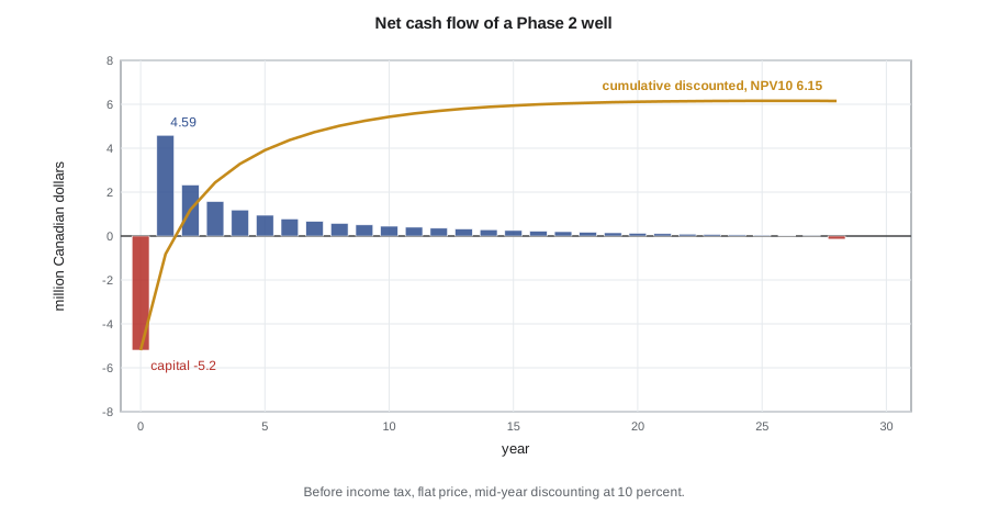
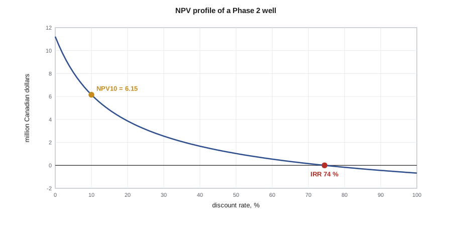
The well produces for 28 years to its economic limit, with an EUR of about 45,300 m³, a little more than the 42,800 m³ of the type well because the cash flow sets a slightly later limit than the 1 m³/d of Lesson 4. The first year earns 4.59 million dollars, nearly the whole capital cost, and the second year 2.33 million. The undiscounted net cash flow is 11.2 million and the NPV10 is 6.15 million. The IRR is 74 percent, payout takes 1.3 years, and the profit-to-investment ratio, NPV10 divided by capital, is 1.18. The capital cost per unit of EUR, about 115 dollars per m³, is a quick measure of capital efficiency that can be compared directly with the netback per m³.
Plotting NPV against discount rate gives the NPV profile. It starts at the undiscounted value at zero percent, falls as the rate rises, and crosses zero at the IRR. For a typical project with capital first and revenue later the profile falls steadily, so a project with a positive NPV at the company's discount rate also has an IRR above that rate. Profiles of different projects can cross, which is why the two measures can rank projects differently; Lesson 9 returns to this.
Worked problem
Payout
The well costs 5.2 million dollars at time zero and earns 4.59 million in year 1 and 2.33 million in year 2. Assuming cash arrives evenly through each year, when does the well pay out?
Show solution
- After year 1 the cumulative cash flow is −5.20 + 4.59 = −0.61 million.
- The remaining 0.61 million is recovered in 0.61 / 2.33 = 0.26 of year 2.
- Payout is 1 + 0.26 = 1.3 years.
Answer: Payout measures how quickly capital is at risk, not how much value the well creates; a well can pay out fast and still have a modest NPV.
Checking a model
Cash flow models fail in predictable ways, and a few checks catch most errors. Units first: a model that mixes daily rates and monthly volumes, or barrels and cubic metres, can be wrong by a factor of 30 or 6.3 and still look reasonable. Interests second: royalties should be applied to revenue, and capital and operating costs to the working interest. Third, totals should reconcile: the sum of the production column should equal the EUR in the reserves table, and the undiscounted cash flow should equal revenue less all costs.
Reasonableness checks come last. Ethan compares the model's operating cost per unit of production in the first and last years with the actual costs of similar wells, the capital cost with recent authorizations for expenditure, the netback with the company's reported netbacks, and the profile with the type curve. He also checks the economic limit year against the age at which older wells in the pool have actually been shut in. A model that passes its arithmetic checks but predicts that wells produce for 50 years when the oldest wells in the play have stopped at 20 is wrong in a way no formula will reveal.
Finally, every model should be tested for sensitivity. Changing one input at a time by a reasonable amount, such as price by 20 percent, EUR by the P90 to P10 range, capital by 15 percent and operating cost by 20 percent, shows which assumptions matter. For new horizontals, EUR and price usually dominate; for mature properties near their limits, operating cost and abandonment matter most. Lesson 11 extends this to tornado charts and Monte Carlo simulation of value.
Common mistakes
MistakeApplying royalties to the working-interest share of costs, or costs to the net revenue interest.
InsteadRevenue and royalties follow the net revenue interest; costs follow the working interest.
MistakeUsing only variable operating costs.
InsteadInclude fixed costs; they set the economic limit and the reserves.
MistakeLeaving out abandonment and reclamation.
InsteadInclude them; they can make mature properties worth less than nothing.
MistakeAccepting a model because the arithmetic checks.
InsteadTest the results against actual costs, netbacks and the field's history.
Summary and key terms
- A cash flow model runs from production through revenue, royalties, operating costs, capital and abandonment to net cash flow.
- Revenue and royalties follow the net revenue interest; costs follow the working interest.
- Fixed operating costs set the economic limit and therefore the reserves.
- NPV, IRR, payout and the profit-to-investment ratio summarize a cash flow.
- The NPV profile crosses zero at the IRR; profiles of different projects can cross.
- Models need unit, interest, reconciliation, reasonableness and sensitivity checks.
- Net cash flow
- Revenue minus royalties, taxes, operating costs, capital and abandonment in a period.
- Internal rate of return (IRR)
- The discount rate at which NPV is zero.
- Payout
- The time for cumulative net cash flow to recover the capital invested.
- Profit-to-investment ratio (PIR)
- NPV divided by capital invested.
- NPV profile
- A plot of NPV against discount rate.
- Fixed operating cost
- Operating cost that does not vary with production rate.
- Abandonment and reclamation
- The costs of plugging a well and restoring the land at the end of its life.
Practice problems
Work each problem on paper first, then reveal the answer to check.
A well earns 3 million in year 1 and 2 million in year 2, and costs 4 million at time zero. When does it pay out?
Show answer
After year 1 it is 1 million short; 1/2 = 0.5, so payout is 1.5 years.
Why does the fixed operating cost affect the reserves?
Show answer
It sets the rate at which revenue no longer covers costs, which is the economic limit.
A project has an NPV10 of 3 million on 12 million of capital. What is its PIR?
Show answer
0.25.
Name three reasonableness checks on a cash flow model.
Show answer
Operating cost per unit versus actual, capital versus recent AFEs, netback versus reported netbacks, economic life versus field history.
Lesson quiz · 5 questions
Score 60% or more to complete this lesson.
Create a free account to save your progress, take quizzes and earn a certificate.