Price forecasts and the time value of money

With forecasts of production in hand, Ethan turns to the other half of value: what the oil and gas will sell for, and how much less a dollar received in the future is worth than a dollar today. Diane gives him the company's price file, which holds three different price forecasts. “One for the reserves report, one for the bank, and one for the budget. They answer different questions, and you have to know which one you are using.” This lesson covers price benchmarks and differentials, how forecasts are built and escalated, and the mathematics of discounting, including the conventions that make two correct calculations disagree.

From benchmark to field price

Crude oil is priced against benchmarks traded in large, liquid markets. The North American benchmark is West Texas Intermediate (WTI) delivered at Cushing, Oklahoma, quoted in US dollars per barrel; the international benchmark is Brent. Canadian light oil is priced at Edmonton, where light sweet crude trades at a differential to WTI that reflects pipeline capacity to US markets and quality. Heavy oil is priced as Western Canadian Select at Hardisty, at a much wider discount. Natural gas in Alberta is priced at the AECO hub in Canadian dollars per gigajoule, and in the United States at Henry Hub, Louisiana.

The price that matters for a well is the field price: the benchmark adjusted for the exchange rate, the location differential, quality adjustments for density and sulphur, and transport from the well to the sales point. For Prairie Crest, Edmonton light sweet is close to the Cardium crude quality, so the field price is the WTI price, less a light-oil differential of about 4.50 US dollars per barrel, converted to Canadian dollars and to cubic metres, less a small trucking and pipeline tariff. The exchange rate has a large effect: a weaker Canadian dollar raises the Canadian-dollar price of oil that is sold in US dollars.

Forecasts for different purposes

NI 51-101 requires reserves and their value to be reported using forecast prices and costs. Most Canadian companies use the price forecast of their independent evaluator, and evaluation firms publish their forecasts each quarter; some companies use an average of the forecasts of several major firms. These decks give a price for each of the next several years, usually close to the futures strip in the first year or two and then rising slowly to a long-term price that is held constant in real terms and escalated at about 2 percent per year. Value under constant prices may also be disclosed but is optional.

Lenders use a third forecast. Banks set their own price deck for borrowing base reviews, usually below the futures strip, because they want the loan to be repaid even if prices fall. The company's budget and long-range plan may use yet another deck chosen by management, often a deliberately conservative flat price. None of these is wrong; they are designed for different purposes. The errors come from mixing them, for example by quoting the value at forecast prices next to the reserves estimated at a lower price.

Escalation, inflation and real values

A forecast can be expressed in nominal dollars, the actual dollars expected in each future year, or in real dollars of constant purchasing power. Evaluations in the industry are normally done in nominal terms: prices and costs are escalated, usually at an assumed inflation rate of about 2 percent per year after the first few years, and the cash flows are discounted at a nominal discount rate. The alternative, real prices and costs discounted at a real rate, gives the same answer if done consistently. The relationship between the two rates is

where f is the inflation rate. A 10 percent nominal rate with 2 percent inflation is equivalent to a real rate of 7.84 percent. The most common error is to escalate prices but not costs, or the reverse, which builds a steady improvement or deterioration in margins into the forecast without anyone deciding it. Costs in the oil industry do not always follow general inflation; drilling and service costs rise when activity is high and fall in downturns, often with a lag behind oil prices.

The script below builds the field price for the Cardium oil from a WTI forecast, exchange rate forecast and differential, escalates it after the fifth year, and compares discount factors and conventions.

# Price decks and the time value of money: escalation, exchange rate, differentials and discount factors.
SI = True      # True: Canadian light oil in Canadian dollars per m3, False: Williston Basin oil in US dollars per bbl
BBL = 6.2898
wti = [64.0, 66.0, 68.0, 70.0, 71.5]            # WTI forecast, US dollars per bbl (illustrative, nominal)
esc = 0.02                                      # escalation after the last forecast year
fx = [0.73, 0.74, 0.75, 0.76, 0.76]             # US dollars per Canadian dollar
diff_ca = 4.5                                   # Edmonton light discount to WTI, US dollars per bbl
diff_us = 5.0                                   # wellhead discount to WTI, US dollars per bbl
years = 10
prices = []
for y in range(years):
    w = wti[y] if y < len(wti) else wti[-1] * (1 + esc) ** (y - len(wti) + 1)
    if SI:
        f = fx[min(y, len(fx) - 1)]
        prices.append((w, (w - diff_ca) / f * BBL))     # Canadian dollars per m3
    else:
        prices.append((w, w - diff_us))                  # US dollars per bbl
unit = "C dollars/m3" if SI else "US dollars/bbl"
print("year   WTI   field price (" + unit + ")")
for y, (w, p) in enumerate(prices, 1):
    if y <= 6 or y == years: print(f"{y:4d} {w:6.1f}  {p:9.1f}")
infl = 0.02
real = [p / (1 + infl) ** (y + 0.5) for y, (_, p) in enumerate(prices)]
print(f"year-10 price in today's money at 2 percent inflation: {real[-1]:.1f} {unit}")
for r in (0.05, 0.10, 0.15):
    end = 1 / (1 + r) ** 10; mid = 1 / (1 + r) ** 9.5; cont = 2.718281828 ** (-r * 9.5)
    print(f"r = {r:.0%}: year-10 discount factor end-year {end:.3f}, mid-year {mid:.3f}, continuous {cont:.3f}")
nominal, inflation = 0.10, 0.02
print(f"real discount rate equivalent to 10 percent nominal: {(1 + nominal) / (1 + inflation) - 1:.4f}")

year   WTI   field price (C dollars/m3)
   1   64.0      512.7
   2   66.0      522.7
   3   68.0      532.5
   4   70.0      542.1
   5   71.5      554.5
   6   72.9      566.3
  10   78.9      616.1
year-10 price in today's money at 2 percent inflation: 510.4 C dollars/m3
r = 5%: year-10 discount factor end-year 0.614, mid-year 0.629, continuous 0.622
r = 10%: year-10 discount factor end-year 0.386, mid-year 0.404, continuous 0.387
r = 15%: year-10 discount factor end-year 0.247, mid-year 0.265, continuous 0.241
real discount rate equivalent to 10 percent nominal: 0.0784

The field price rises from about 513 Canadian dollars per m³ in the first year to 616 in year ten. In today's money, at 2 percent inflation, the year-ten price is about 510 dollars, essentially the same as today's: the deck is flat in real terms after the first few years, which is typical of evaluators' long-term assumptions.

Discounting conventions

The discount factor for a cash flow received t years after the effective date at an annual rate i is 1/(1 + i)^t. The question is what t should be. If each year's cash flow is treated as arriving at the end of the year, the first year's cash flow is discounted by a full year, which undervalues it because production and sales occur throughout the year. The mid-year convention treats each year's cash flow as arriving in the middle of the year, t − 0.5 for year t, which is closer to reality for steady monthly revenue. Some software uses continuous discounting, e^(−it), with the same timing choices, or discounts monthly cash flows directly.

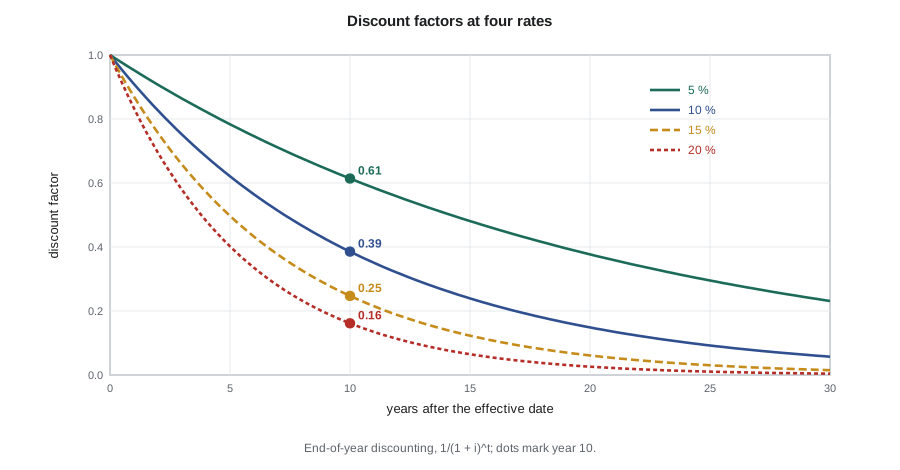
The differences between conventions are not trivial for front-loaded production. In the script, the year-ten discount factor at 10 percent is 0.386 with end-year timing and 0.404 with mid-year timing, a 5 percent difference, and for the first year the difference is the same 5 percent on a much larger cash flow. A reader comparing two evaluations must know which convention each used. Reserves reports state the convention, and most use mid-year or monthly discounting.

Choosing the discount rate

The discount rate represents the return the company could earn on alternative uses of its money, adjusted for risk. Companies often use their weighted average cost of capital, the blended cost of their debt and equity, as a base, and may add premiums for riskier projects. Because readers of a reserves report have different views, reports present values at several rates: NPV0 shows the undiscounted total, and NPV10 is the most quoted single figure, partly because the SEC's standardized measure and many lenders use 10 percent. Higher rates penalize long-lived projects such as waterfloods and EOR schemes more than short-lived ones such as new horizontals, so the ranking of projects can depend on the rate chosen, a point that returns in Lesson 9.

Ethan notices that changing the discount rate from 10 to 15 percent lowers the value of the Phase 2 well by a fifth to a quarter, while changing the long-term oil price by 10 percent changes it by a similar amount. Price and discount rate are the two economic assumptions to which value is most sensitive, and both are partly matters of judgement. That is why reports show values at several discount rates, and why companies test their plans against low and high price cases.

Gas prices, liquids and hedging

Gas and natural gas liquids need their own price forecasts. AECO gas prices are set by supply and demand in western Canada and by pipeline capacity to other markets, and have at times traded at a deep discount to Henry Hub; liquefied natural gas exports from the British Columbia coast, which began in mid-2025, are strengthening the link to international markets. Liquids such as propane, butane and pentanes plus are priced relative to crude oil or to regional hubs, and pentanes plus, used as diluent for heavy oil, often trades close to light oil prices. For a light oil producer like Prairie Crest, gas and liquids add a modest share of revenue, but in liquids-rich gas plays they can provide more than half.

Many companies hedge part of their production with swaps, collars or put options, fixing or bounding the price for the next one or two years. Hedges protect cash flow and the capital program from a price collapse, and lenders often require them. In a reserves evaluation, however, hedges are usually excluded from the value of the reserves and reported separately, because they are financial contracts rather than properties of the reserves. An evaluator should state clearly whether a value includes hedges, and Ethan's cash flow models leave them out. The same logic applies to other contracts that change the realized price, such as marketing arrangements or firm transport commitments: they belong in the evaluation only if they are tied to the production and will continue over the life of the reserves, and their terms should be documented. Firm transport that the company must pay for whether or not it ships is a cost that can outlast the production it was meant to carry, so Ethan checks that its fees are included in the operating costs for as long as the contracts run.