
PET-360 · Lesson 8 of 12 · 16 min
Naturally fractured and layered reservoirs
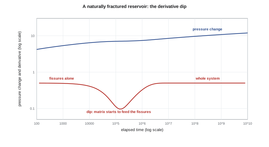
The east side of the pool includes an older vertical well completed in a fractured carbonate below the Cardium. Its buildup, which nobody has interpreted properly, shows a derivative that starts flat, dips into a deep valley and then climbs back to a second flat level at the same height. Ethan suspects a bad gauge. Lena, who worked in carbonates for ten years, recognizes it at once. 'That is a textbook dual-porosity dip,' she says. 'The fractures carry the flow, and the rock between them holds the oil. The valley is the moment the matrix wakes up.'
This lesson covers reservoirs with two interacting media: naturally fractured rock modelled with the Warren and Root dual-porosity model, the storativity ratio ω and the interporosity flow coefficient λ, the different forms of matrix-to-fracture flow, and the closely related behaviour of layered reservoirs with and without crossflow. It also covers composite reservoirs, where properties change with distance from the well.
Two porosities, one flow path
Many carbonates, some tight sandstones and most basement reservoirs contain natural fractures. The fractures have little pore volume but high permeability; the matrix blocks between them hold most of the fluid but have low permeability. In 1963, Warren and Root proposed an idealized model: the reservoir is a regular array of matrix blocks separated by fractures, fluid flows to the well only through the fractures, and the matrix feeds the fractures locally. The model reduces the complex geometry to two parameters beyond the usual kh and skin.
The storativity ratio ω is the fraction of the total storage in the fractures, typically 0.001 to 0.1. The interporosity flow coefficient λ measures how easily fluid moves from matrix to fractures; α is a shape factor that depends on the block geometry and size, so small blocks and permeable matrix give large λ. Values usually lie between 10⁻⁹ and 10⁻³. Here k_f is the bulk fracture permeability, which is what the test measures as k.
The three periods of a dual-porosity test
At early time, only the fractures respond. The pressure falls quickly because the fractures hold little fluid, and the well behaves like a homogeneous reservoir with storage (φc_t)_f: the derivative shows a first radial-flow plateau. Then the pressure drop in the fractures becomes large enough to draw fluid from the matrix. The extra supply slows the pressure decline, so the derivative dips. Finally, the matrix and fractures come into equilibrium, and the system behaves like a homogeneous reservoir with the total storage: a second plateau at the same level, because the flow still goes only through the fractures and kh has not changed.
On a semilog plot, the two radial-flow periods give two parallel straight lines with the same slope m. The vertical separation between them depends only on ω: it equals m log(1/ω). The timing of the transition depends on λ: a small λ delays the dip, while a large λ brings it so early that it may be hidden under wellbore storage.
# A naturally fractured (dual-porosity) reservoir: the derivative dip, and omega and lambda from it
import math
SI = True
def I0(x):
    t = x / 3.75
    if x <= 3.75:
        y = t * t
        return 1 + y * (3.5156229 + y * (3.0899424 + y * (1.2067492 + y * (0.2659732 + y * (0.0360768 + y * 0.0045813)))))
    y = 1 / t
    return math.exp(x) / math.sqrt(x) * (0.39894228 + y * (0.01328592 + y * (0.00225319 + y * (-0.00157565 + y * (0.00916281 + y * (-0.02057706 + y * (0.02635537 + y * (-0.01647633 + y * 0.00392377))))))))
def I1(x):
    t = x / 3.75
    if x <= 3.75:
        y = t * t
        return x * (0.5 + y * (0.87890594 + y * (0.51498869 + y * (0.15084934 + y * (0.02658733 + y * (0.00301532 + y * 0.00032411))))))
    y = 1 / t
    return math.exp(x) / math.sqrt(x) * (0.39894228 + y * (-0.03988024 + y * (-0.00362018 + y * (0.00163801 + y * (-0.01031555 + y * (0.02282967 + y * (-0.02895312 + y * (0.01787654 - y * 0.00420059))))))))
def K0(x):                       # modified Bessel functions by polynomial approximations
    if x <= 2:
        y = x * x / 4
        return -math.log(x / 2) * I0(x) - 0.57721566 + y * (0.42278420 + y * (0.23069756 + y * (0.03488590 + y * (0.00262698 + y * (0.00010750 + y * 0.0000074)))))
    y = 2 / x
    return math.exp(-x) / math.sqrt(x) * (1.25331414 + y * (-0.07832358 + y * (0.02189568 + y * (-0.01062446 + y * (0.00587872 + y * (-0.00251540 + y * 0.00053208))))))
def K1(x):
    if x <= 2:
        y = x * x / 4
        return math.log(x / 2) * I1(x) + (1 / x) * (1 + y * (0.15443144 + y * (-0.67278579 + y * (-0.18156897 + y * (-0.01919402 + y * (-0.00110404 - y * 0.00004686))))))
    y = 2 / x
    return math.exp(-x) / math.sqrt(x) * (1.25331414 + y * (0.23498619 + y * (-0.03655620 + y * (0.01504268 + y * (-0.00780353 + y * (0.00325614 - y * 0.00068245))))))
def stehfest(F, t, N=12):         # numerical inversion of a Laplace-space function F(s) at time t
    ln2 = math.log(2); total = 0.0
    for i in range(1, N + 1):
        v = 0.0
        for k in range((i + 1) // 2, min(i, N // 2) + 1):
            v += k ** (N // 2) * math.factorial(2 * k) / (math.factorial(N // 2 - k) * math.factorial(k) * math.factorial(k - 1) * math.factorial(i - k) * math.factorial(2 * k - i))
        total += (-1) ** (i + N // 2) * v * F(i * ln2 / t)
    return total * ln2 / t

omega, lam = 0.05, 1e-6            # storativity ratio and interporosity flow coefficient (pseudosteady matrix flow)
def pD_lap(u):                     # Warren-Root solution in Laplace space, line source, no skin or storage
    f = (omega * (1 - omega) * u + lam) / ((1 - omega) * u + lam)
    return K0(math.sqrt(u * f)) / u
tDs = [1e3 * 1.5 ** i for i in range(42)]
pD = [stehfest(pD_lap, t) for t in tDs]
der = [(pD[i + 1] - pD[i - 1]) / math.log(tDs[i + 1] / tDs[i - 1]) for i in range(1, len(tDs) - 1)]
print("      tD        pD     derivative")
for i in range(1, len(tDs) - 1, 4):
    print(f"{tDs[i]:10.3g}  {pD[i]:7.3f}   {der[i - 1]:7.3f}")
i_min = min(range(len(der)), key=lambda i: der[i])
print(f"derivative minimum {der[i_min]:.3f} at tD = {tDs[i_min + 1]:.3g}")
print(f"approximate prediction for the minimum: tD = (omega/lambda) ln(1/omega) = {omega / lam * math.log(1 / omega):.3g}")
# separation of the two parallel semilog lines (each with slope 1.151 in pD per log cycle)
early = 0.5 * (math.log(tDs[3] / omega) + 0.80907); late_line = 0.5 * (math.log(tDs[3]) + 0.80907)
dp_sep = early - late_line
print(f"vertical separation of the parallel lines: {dp_sep:.3f} in pD = {dp_sep / 1.1513:.3f} log cycles")
print(f"omega recovered from the separation: {10 ** (-dp_sep / 1.1513):.3f}")
if SI: print("in a well with m = 120 kPa/cycle that separation would be about", round(dp_sep / 1.1513 * 120), "kPa")
else: print("in a well with m = 70 psi/cycle that separation would be about", round(dp_sep / 1.1513 * 70), "psi")tD pD derivative 1.5e+03 5.544 0.485 7.59e+03 6.297 0.429 3.84e+04 6.865 0.242 1.95e+05 7.094 0.106 9.85e+05 7.408 0.323 4.99e+06 8.116 0.496 2.53e+07 8.927 0.500 1.28e+08 9.738 0.500 6.47e+08 10.549 0.500 3.28e+09 11.360 0.500 derivative minimum 0.102 at tD = 1.3e+05 approximate prediction for the minimum: tD = (omega/lambda) ln(1/omega) = 1.5e+05 vertical separation of the parallel lines: 1.498 in pD = 1.301 log cycles omega recovered from the separation: 0.050 in a well with m = 120 kPa/cycle that separation would be about 156 kPa
The derivative dips from 0.5 to about 0.10 at a dimensionless time of 1.3 × 10⁵ and recovers by 2.5 × 10⁷. The simple estimate (ω/λ) ln(1/ω) predicts the minimum at 1.5 × 10⁵, close enough for planning. The separation of the two semilog lines is 1.30 log cycles, which gives back ω = 0.05 exactly. In a well with a slope of 120 kPa per cycle, that separation would be about 156 kPa, large enough to see easily.
Pseudosteady and transient matrix flow
Warren and Root assumed that the matrix delivers fluid to the fractures in pseudosteady state: the pressure inside each block is uniform and drops in step with the fracture pressure. This gives the sharp V-shaped valley above. Other workers, including Kazemi and de Swaan in the 1970s, modelled transient flow inside the blocks. Transient matrix flow gives a shallower, wider transition, and in the middle of it the derivative can settle on a plateau at half the radial level, because the matrix contributes as if it were a second medium in parallel. In practice the two forms are hard to tell apart unless the data are excellent, and the parameters ω and λ estimated with either model are usually close enough for engineering use.
When the dip is not a fracture system
The same derivative valley appears in a layered reservoir with crossflow, where a thin high-permeability layer responds first and then draws fluid from thicker low-permeability layers. Mathematically the problem is almost identical to dual porosity. Without crossflow, where shale barriers separate the layers and they communicate only through the wellbore, the response is different: early on, the layers behave like a single reservoir with the total kh, but differences in boundary distance or depletion between layers can produce confusing late-time shapes, and the wellbore can carry fluid from one layer to another during a shut-in. Production logs that measure the rate from each layer, or a layered test with packers, are the usual way to separate them.
A composite reservoir has one set of properties near the well and another farther out: for example, an inner region swept by injected water, a zone of different facies, or an area near a fault where natural fractures are more intense. The derivative shows two plateaus at different levels. The ratio of the levels gives the ratio of mobilities, and the transition time gives the distance to the change. A step up means lower mobility outside; a step down means higher mobility outside. A step up of exactly twice is indistinguishable from a sealing fault without other information.
| Response | Model | What the parameters mean |
|---|---|---|
| Flat, valley, flat at the same level | Dual porosity (Warren and Root) | Depth gives ω; timing gives λ |
| Flat, shallow plateau at half level, flat | Dual porosity with transient matrix flow | Same parameters with a different matrix model |
| Similar valley in clastics with known layers | Layered reservoir with crossflow | Thin permeable layer fed by tight layers |
| Two plateaus at different levels | Radial composite | Level ratio gives mobility ratio; timing gives distance |
| Erratic late behaviour, layers isolated | Layered without crossflow | Use production logs or isolated layer tests |
Why the parameters matter
In a dual-porosity reservoir, ω tells the engineer how much of the fluid is in the fractures. A small ω means the fractures hold little and early production may decline fast before the matrix supports it. λ indicates how quickly the matrix gives up its fluid, which affects rate decline and, in water-drive or gas-cap reservoirs, how quickly fractures can carry water or gas to the well ahead of the oil in the matrix. Fractured reservoirs are notorious for early water breakthrough through fracture corridors while much of the matrix oil is bypassed, so a test that identifies dual-porosity behaviour early changes development decisions about rate, completion depth and pressure maintenance.
Worked problem
Estimating ω from a field buildup
A buildup in the fractured carbonate well shows two parallel semilog lines, each with a slope of 95 kPa per cycle, separated vertically by 140 kPa. What is ω, and what does it mean?
Show solution
- The separation equals m log(1/ω), so log(1/ω) = 140/95 = 1.47.
- 1/ω = 10^1.47 ≈ 30, so ω ≈ 0.034.
- About 3 percent of the total storage is in the fractures; the matrix holds the rest.
Answer: Most of the oil is in the matrix, so long-term recovery depends on how well the matrix feeds the fractures, and the λ from the transition time is the next number to estimate.
Common mistakes
MistakeMistaking a dual-porosity dip for gauge noise or a bad test.
InsteadCheck the shape against the Warren and Root model and the geology.
MistakeReading the first plateau as the only kh.
InsteadBoth plateaus give the same kh; the second confirms it.
MistakeAssuming a valley always means natural fractures.
InsteadLayered reservoirs with crossflow show the same shape; use cores, logs and production logs.
MistakeExpecting to see the dip in every fractured well.
InsteadA large λ hides the transition under wellbore storage; a small λ may push it past the test.
MistakeTreating a two-level step as a fault without checking.
InsteadA radial composite can give the same response; look for supporting geology.
Summary and key terms
- Warren and Root represent fractured rock by fractures that carry flow and matrix blocks that store fluid.
- The storativity ratio ω is the fraction of storage in the fractures; λ measures matrix-to-fracture flow.
- The derivative shows a plateau, a valley and a second plateau at the same level.
- The parallel semilog lines are separated by m log(1/ω); the transition time depends on λ.
- Layered reservoirs with crossflow can produce the same shape as dual porosity.
- Radial composite reservoirs show two plateaus at different levels, related to mobility ratio.
- Dual porosity
- A reservoir model with two interacting media, typically fractures and matrix.
- Storativity ratio ω
- The fraction of the total storage (φc_t) contained in the fractures.
- Interporosity flow coefficient λ
- A dimensionless measure of how easily the matrix delivers fluid to the fractures.
- Layered reservoir with crossflow
- A reservoir of several layers in vertical communication.
- Radial composite
- A reservoir with different properties inside and outside a circle around the well.
- Mobility
- Permeability divided by viscosity, k/μ.
Practice problems
Work each problem on paper first, then reveal the answer to check.
Why are the two plateaus at the same level in a dual-porosity test?
Show answer
Flow to the well goes only through the fractures, so kh is the same.
What does a small ω mean?
Show answer
Little of the storage is in the fractures.
What delays the dual-porosity transition?
Show answer
A small λ, from large blocks or tight matrix.
What other model can produce a dual-porosity valley?
Show answer
A layered reservoir with crossflow.
Lesson quiz · 5 questions
Score 60% or more to complete this lesson.
Create a free account to save your progress, take quizzes and earn a certificate.