
PET-360 · Lesson 7 of 12 · 19 min
Boundaries and reservoir limits
Mei Lin's seismic interpretation of Prairie Crest shows a small normal fault running north-south about 150 m east of the 100/08-27 delineation well. Nobody knows whether it seals. If it does, the delineation well sits in a narrower block than the development plan assumes, and two of the planned wells move. 'Can the test tell us?' Tom Ashworth asks at the planning meeting. Ethan, who has spent the last month on derivatives, says yes, if the well flows long enough for the pressure transient to reach the fault and come back.
This lesson covers how boundaries appear in well tests: the radius of investigation, the method of images for sealing faults, channels and intersecting faults, constant-pressure boundaries, closed drainage areas and pseudosteady state, and the reservoir limit test that measures the connected volume. Boundaries are the late-time part of the diagnostic plot, and they matter commercially because they control how much oil or gas one well can reach.
How far does a test see?
A pressure disturbance spreads outward from the well by diffusion. The radius of investigation is a measure of how far it has travelled after a given time. A widely used definition takes the radius at which the pressure disturbance from an impulse is largest, giving in oilfield units:
Here r_i is in feet, k in millidarcies, t in hours, μ in centipoise and c_t in reciprocal psi. The metric form, with r_i in metres, t in hours and c_t in reciprocal kilopascals, has a constant of about 70,350 in place of 948 when k is in millidarcies and μ in mPa·s. The radius grows with the square root of time: to see twice as far, a test must run four times as long. It also grows with the square root of the diffusivity k/(φμc_t), which is why a test in a tight rock sees only a short distance in the same time, a point that returns in lesson 9.
The radius of investigation is a rule of thumb, not a sharp edge. Pressure changes extend beyond it, just too small to measure, and a boundary at r_i affects the test only slightly at that moment. To identify a boundary clearly, the data should continue until the radius is two or three times the distance to it. The test must also have a clean radial-flow period first, because a boundary is recognized by how the response departs from radial flow.
Sealing faults and image wells
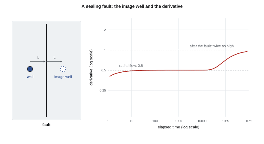
A straight sealing fault blocks flow across a line. The mathematical trick for this case is the method of images: the pressure in a reservoir with a straight no-flow boundary is the same as in an infinite reservoir with a second, imaginary well placed symmetrically on the other side of the fault, producing at the same rate. By symmetry, no flow crosses the line midway between the real and image wells, which is exactly the fault condition. The pressure drop at the real well is the sum of its own drop and the drop caused by the image well at a distance 2L, where L is the distance to the fault.
Early on, the image term is zero and the well behaves as if the fault did not exist. Once the transient reaches the fault, the image term grows, and at late time it adds the same logarithmic increase as the real well. The semilog slope therefore doubles, from m to 2m, and the derivative rises from its radial-flow level to twice that level. That doubling is the classic signature of a single sealing fault.
The distance to the fault can be estimated from the time at which the two semilog straight lines intersect, t_x. A common formula, given by Gray in the 1960s, is:
with L in feet, t_x in hours and the other quantities in oilfield units. The constant combines the 948 of the radius equation with the factor 1.781, the exponential of Euler's constant, which appears when the two logarithmic lines are set equal, and a factor of one half because the image well sits at 2L. In practice, software fits L directly by regression on the full image-well model, which uses all the data rather than one intersection.
# A sealing fault seen in a drawdown: image-well superposition, the derivative doubling, and the fault distance
import math
SI = True
def E1(x):
    if x > 8: return math.exp(-x) / x * (1 - 1 / x + 2 / x ** 2)     # asymptotic form for large x
    g, total, term = 0.5772156649, 0.0, 1.0
    for n in range(1, 80):
        term *= -x / n
        total += -term / n
    return -g - math.log(x) + total
if SI:   # metric units
    q, B, mu, h, phi, ct, rw, k, s, L = 5.5, 1.29, 0.72, 6.5, 0.14, 1.5e-6, 0.089, 15.0, 5.0, 150.0
    c_pD, c_tD, c_m, pu, lu = 1866.6, 3.553e-6, 2149.3, "kPa", "m"
else:
    q, B, mu, h, phi, ct, rw, k, s, L = 300.0, 1.25, 0.90, 30.0, 0.12, 1.2e-5, 0.35, 25.0, 5.0, 500.0
    c_pD, c_tD, c_m, pu, lu = 141.2, 2.637e-4, 162.6, "psi", "ft"
A = c_pD * q * B * mu / (k * h); eta = c_tD * k / (phi * mu * ct)     # eta: diffusivity per hour
def dp(t):          # the producing well plus an image well at distance 2L across the fault
    return A * (0.5 * E1(rw ** 2 / (4 * eta * t)) + s + 0.5 * E1((2 * L) ** 2 / (4 * eta * t)))
times = [0.5 * 1.25 ** i for i in range(40)]
vals = [dp(t) for t in times]
der = [(vals[i + 1] - vals[i - 1]) / (math.log(times[i + 1]) - math.log(times[i - 1])) for i in range(1, len(times) - 1)]
print("   t (h)    dp     t*dp/dt")
for i in range(1, len(times) - 1, 4):
    print(f"{times[i]:8.1f} {vals[i]:7.1f}  {der[i - 1]:7.1f}")
m1 = c_m * q * B * mu / (k * h)
print(f"first semilog slope {m1:.1f} {pu}/cycle; after the fault it doubles to {2 * m1:.1f}")
# intersection of the two semilog straight lines gives t_x
early = [(math.log10(t), v) for t, v in zip(times, vals) if 2 < t < 6]
late = [(math.log10(t), v) for t, v in zip(times, vals) if t > 2000]
def fit(p):
    n = len(p); sx = sum(a for a, _ in p); sy = sum(b for _, b in p)
    sxx = sum(a * a for a, _ in p); sxy = sum(a * b for a, b in p)
    m = (n * sxy - sx * sy) / (n * sxx - sx * sx); return m, (sy - m * sx) / n
(m_e, b_e), (m_l, b_l) = fit(early), fit(late)
tx = 10 ** ((b_e - b_l) / (m_l - m_e))
L_est = math.sqrt(eta * tx / 1.781)
print(f"slopes fitted: {m_e:.1f} and {m_l:.1f} {pu}/cycle; lines cross at t_x = {tx:.0f} h")
print(f"estimated distance to the fault = {L_est:.0f} {lu} (true {L:.0f} {lu})") t (h) dp t*dp/dt
0.6 1029.0 48.9
1.5 1072.6 48.9
3.7 1116.2 48.9
9.1 1159.9 49.0
22.2 1204.3 51.8
54.2 1255.2 64.0
132.3 1319.3 79.0
323.1 1394.8 89.0
788.9 1476.7 94.0
1925.9 1561.7 96.2
first semilog slope 112.6 kPa/cycle; after the fault it doubles to 225.2
slopes fitted: 112.6 and 222.5 kPa/cycle; lines cross at t_x = 103 h
estimated distance to the fault = 143 m (true 150 m)The synthetic test reproduces the expected behaviour. The derivative stays at 49 kPa until about 10 hours, starts to rise near 20 hours and approaches twice its earlier level by about 2,000 hours. The two fitted semilog slopes are 113 and 223 kPa per cycle, and their intersection at about 103 hours gives a fault distance of 143 m, within 5 percent of the 150 m used to build the data. Ethan notes the catch: the flow needed to show the doubling clearly is weeks long, and a 72-hour buildup would show only the start of the rise.
Channels, intersecting faults and partial seals
More complex boundaries are handled by more image wells. Two parallel sealing faults form a channel, which needs an infinite row of images; once both sides are felt, flow becomes linear along the channel and the derivative climbs on a half slope. Channels are common in fluvial sands and in narrow reef trends. Two faults that intersect at an angle form a wedge: for a wedge of angle θ, the late derivative rises to 360/θ times the radial level, so a 90 degree corner gives four times, and the well sits in a quarter of an infinite reservoir. A fault that only partly seals gives a rise smaller than double, and the size of the rise reflects the fault's transmissibility. A change in reservoir properties away from the well, such as a lower-permeability outer region, can give a similar rise; this is the non-uniqueness of lesson 5 in action, and the seismic map is what favours a fault.
Constant-pressure boundaries
A gas cap, a strong aquifer, or a nearby injector can hold pressure nearly constant along a boundary. The image well for a constant-pressure boundary is an injector rather than a producer, so its effect cancels the real well's late pressure decline. The pressure stabilizes, and the derivative falls away steeply, toward zero. A falling derivative is good news for production but has a caution attached: in a buildup after a short flow, the derivative can also fall for reasons unrelated to any boundary, so an apparent constant-pressure boundary needs supporting evidence, such as a known gas-oil contact at about the right distance.
Closed reservoirs and pseudosteady state
If the well drains a closed area, the transient eventually reaches all of the boundaries. In a drawdown, the pressure then falls at a uniform rate everywhere in the drainage area, a condition called pseudosteady state. The rate of decline depends only on the connected pore volume:
with A in square feet, t in hours and dp/dt in psi per hour. On the diagnostic plot, the drawdown derivative bends onto a unit slope at late time, because a pressure falling linearly in time gives a derivative proportional to time. In a buildup, the same closed system makes the derivative fall toward zero as the pressure approaches the average reservoir pressure, which is one reason boundary interpretation from buildups needs care.
A reservoir limit test is a long drawdown run deliberately into pseudosteady state. The slope of pressure against time on a Cartesian plot gives the connected pore volume, φAh, and with porosity and thickness from logs, the drainage area. The test is used in exploration and appraisal wells, where the commercial question is whether the discovery is large enough to develop. It needs a long, stable flow, a facility that can take the production or flare the gas within the permit limits, and a reservoir small enough or permeable enough to reach the boundaries in weeks rather than years.
| Boundary | Late-time derivative (drawdown) | Commercial meaning |
|---|---|---|
| Single sealing fault | Rises to twice the radial level | Smaller block; may affect well spacing |
| Parallel faults (channel) | Half slope | Elongated reservoir; locate wells along the trend |
| Intersecting faults at θ | Rises to 360/θ times the radial level | Well in a wedge or corner |
| Constant-pressure boundary | Falls toward zero | Pressure support from a gas cap or aquifer |
| Closed drainage area | Unit slope (pseudosteady state) | Connected volume can be measured |
Worked problem
How long to see the fault?
Using the 100/08-27 delineation well properties (k = 15 mD, φ = 0.14, μ = 0.72 mPa·s, c_t = 1.5 × 10⁻⁶ kPa⁻¹), how long must the well flow for the radius of investigation to reach three times the 150 m fault distance?
Show solution
- The target radius is 450 m.
- Rearranging the metric radius equation gives t = 70,350 φμc_t r_i²/k.
- t = 70,350 × 0.14 × 0.72 × 1.5 × 10⁻⁶ × 450²/15 ≈ 144 hours, about six days.
Answer: A flow of several days, followed by a buildup of similar length, should show the start of the doubling clearly enough to confirm or rule out a sealing fault.
Common mistakes
MistakeInterpreting a boundary before radial flow is established.
InsteadA boundary is recognized as a departure from radial flow; the flat derivative must come first.
MistakeTreating r_i as a sharp edge.
InsteadRun the test until r_i is two to three times the expected boundary distance.
MistakeCalling every late rise a fault.
InsteadConsider permeability changes and partial seals, and check against seismic.
MistakeCalling every late fall a constant-pressure boundary.
InsteadIn buildups, short flows and redistribution can cause falls; look for independent evidence.
MistakeReading drainage area from a buildup derivative.
InsteadUse a drawdown into pseudosteady state, or model the full history.
Summary and key terms
- The radius of investigation grows with the square root of time and of diffusivity.
- A sealing fault is modelled by an image well; the semilog slope and derivative double.
- The fault distance follows from the intersection time of the two semilog lines, or better by regression.
- Channels give a half slope, wedges a rise to 360/θ times the radial level.
- Constant-pressure boundaries make the derivative fall; closed areas give a late unit slope in drawdowns.
- A reservoir limit test measures connected pore volume from the pseudosteady-state decline.
- Radius of investigation
- The approximate distance a pressure transient has travelled after a given time.
- Method of images
- Representing a boundary by imaginary wells placed so that the boundary condition is satisfied.
- Sealing fault
- A fault that prevents flow across it.
- Channel
- A long narrow reservoir bounded by two parallel no-flow boundaries.
- Pseudosteady state
- Flow in a closed area when pressure declines at the same rate everywhere.
- Reservoir limit test
- A long drawdown designed to reach pseudosteady state and measure connected volume.
Practice problems
Work each problem on paper first, then reveal the answer to check.
How much longer must a test run to see twice as far?
Show answer
Four times as long.
What derivative change does a single sealing fault produce?
Show answer
It doubles.
What does a late unit slope in a drawdown derivative indicate?
Show answer
Pseudosteady state in a closed drainage area.
Which image well represents a constant-pressure boundary?
Show answer
An injector at the mirror position.
Lesson quiz · 5 questions
Score 60% or more to complete this lesson.
Create a free account to save your progress, take quizzes and earn a certificate.