The diffusivity equation and dimensionless variables

Rafael Moreau starts Ethan's training the way he was taught: with a pencil. 'Every interpretation package on your laptop solves one equation,' he says, writing it on the whiteboard in the the Drayton Valley field office. 'If you understand where it comes from and what its assumptions are, you will know when the software is telling you the truth and when it is fitting noise. If you skip this, you will learn to push buttons.' This lesson derives the diffusivity equation for radial flow, introduces the dimensionless variables that make solutions general, and develops the line-source solution that underlies the semilog methods in lessons 3 and 4.

Building the equation

The diffusivity equation combines three physical statements. The first is conservation of mass: in any small volume of rock, the mass flowing in minus the mass flowing out equals the rate at which the mass stored in the pores changes. The second is Darcy's law, from PET-320: the flow velocity is proportional to the pressure gradient, the permeability and the inverse of the viscosity. The third is an equation of state for the fluid and the rock: when pressure falls, the fluid expands and the pore volume shrinks slightly, and the total compressibility c_t measures how much stored fluid is released per unit volume per unit pressure drop.

For a well in the middle of a horizontal, uniform layer, flow is radial, and the natural coordinate is the distance r from the well. Consider a thin ring of rock between r and r + dr, with thickness h. The mass flow rate through the inner face, by Darcy's law, depends on the pressure gradient there; the flow through the outer face depends on the gradient at r + dr. The difference must equal the rate of change of stored mass in the ring, which is the ring's pore volume times the fluid density times c_t times the rate of pressure change. Dividing by the ring volume and letting dr shrink gives a partial differential equation.

This is the radial diffusivity equation. The group k/(φμc_t) is the hydraulic diffusivity, often written η. It plays the same role as the thermal diffusivity in heat conduction: it controls how fast a pressure disturbance spreads. High permeability spreads the disturbance fast; high viscosity, porosity or compressibility slow it down. The radius of investigation in lesson 1 is simply the square root of η times time, with a constant.

The assumptions behind it

The equation above is linear in pressure, which is what makes the rest of well testing possible, but it is linear only because of several assumptions. The rock is homogeneous and isotropic, so k, φ and h are the same everywhere. The layer is horizontal and of uniform thickness, and flow is radial and horizontal. There is a single fluid of small and constant compressibility and constant viscosity. Gravity effects are negligible, and pressure gradients are small enough that the squared-gradient term, which appears when density changes with pressure, can be dropped.

Real reservoirs break some of these assumptions, and much of the rest of this course deals with the ways they do. Gas is highly compressible and its viscosity changes with pressure, so lesson 10 replaces pressure with a pseudopressure that restores linearity. Natural fractures, layers and hydraulic fractures change the geometry (lessons 8 and 9). Boundaries limit the radial extent (lesson 7). Below the bubble point, two phases flow and relative permeability enters; analysts often treat the oil phase alone or use multiphase pseudopressures. The skin factor, introduced in PET-320, gathers all the near-well effects into a single number.

Initial and boundary conditions

An equation alone does not define a problem; it needs conditions. For the basic drawdown problem, the reservoir starts at a uniform initial pressure p_i. At the outer edge, the reservoir is assumed infinite, so the pressure far away stays at p_i. At the well, the well produces at a constant rate q, which by Darcy's law fixes the pressure gradient at the wellbore radius. Different tests change these conditions: a buildup changes the rate at the well, a fault changes the outer condition on one side, and a closed pool replaces the infinite boundary with a no-flow boundary.

Dimensionless variables

Every well has different permeability, thickness, viscosity and rate, so solving the equation separately for each well would be endless. Instead, analysts define dimensionless variables that strip out the units and the well-specific numbers. In oilfield units the three main ones are as follows.

Here q is in stock-tank barrels per day, B in reservoir barrels per stock-tank barrel, μ in centipoise, k in millidarcies, h and r_w in feet, p in psi, t in hours and c_t in reciprocal psi. In the metric units used in Canada, with q in cubic metres per day, h and r_w in metres, p in kilopascals and c_t in reciprocal kilopascals, the constant 141.2 becomes about 1,866.6 and the constant 0.0002637 becomes about 3.553 × 10⁻⁶. Rafael keeps both sets in his notebook because Prairie Crest has wells on both sides of the border.

In these variables the diffusivity equation has no parameters at all, and the constant-rate condition at the well becomes simply ∂p_D/∂r_D = −1 at r_D = 1. A single solution p_D(t_D, r_D) therefore describes every well with the same geometry. To use it for a real well, the engineer converts measured times to t_D and measured pressure changes to p_D, which requires k and the other properties. In practice the logic runs backwards: the shape of the measured response is matched to the dimensionless solution, and the shift between the two gives k and the skin. That is the idea behind type curves (lesson 6) and behind the straight-line methods, which match only one part of the solution.

The line-source solution

For an infinite reservoir and a well so small that it can be treated as a line, the constant-rate problem has an exact solution, first used in petroleum engineering in the late 1940s, building on earlier work in heat conduction and groundwater hydrology. It is written with the exponential integral E₁.

The exponential integral cannot be written with elementary functions, but it is easy to compute. For small arguments a series converges quickly, and for large arguments an asymptotic form works. The code below uses the series. The line source is excellent at the well once t_D is larger than about 25, which for a real well means a few seconds or minutes, and it also gives the pressure at an observation well some distance away, which is the basis of interference testing in lesson 11.

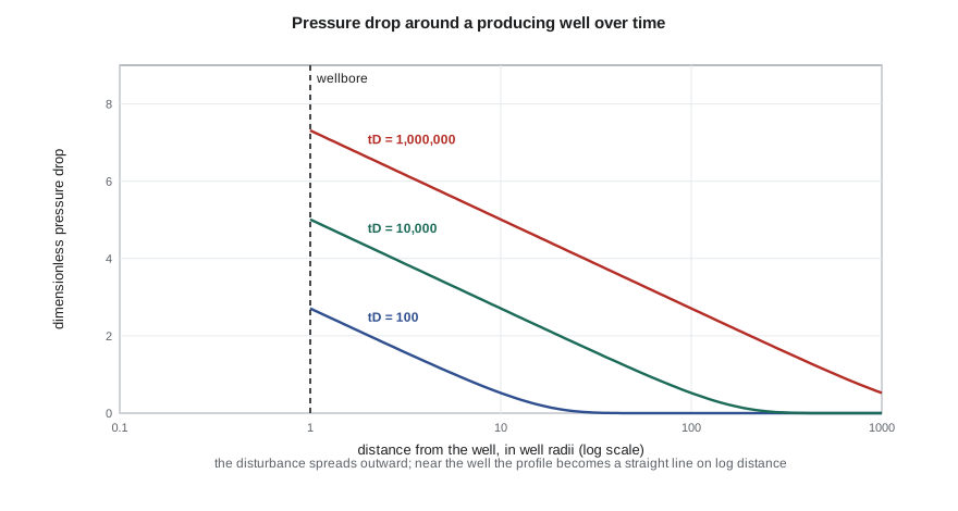
When the argument x = r_D²/(4t_D) is small, which means the disturbance has travelled well past the point of interest, the exponential integral is very close to −ln(x) − 0.5772, where 0.5772 is Euler's constant. Substituting gives the logarithmic approximation that drives most of well testing.

In words: once the disturbance is established, the pressure at a point falls in proportion to the logarithm of time. On a plot of pressure against the logarithm of time, the data fall on a straight line, and the slope of that line depends only on kh and the fluid properties, not on porosity, compressibility or well radius. This is why semilog plots are so powerful, and why permeability is usually the best-determined result of a test.

# The line-source solution: E1 by series, dimensionless pressure, and the log approximation
import math
SI = True   
def E1(x):                                    # exponential integral by its convergent series (fine for x < 10)
    g = 0.5772156649
    total, term = 0.0, 1.0
    for n in range(1, 60):
        term *= -x / n
        total += -term / n
    return -g - math.log(x) + total
print("  tD/rD^2      pD = E1(1/(4tD))/2    log approximation")
for tD in (1, 5, 25, 100, 1000, 1e5):
    exact = 0.5 * E1(1 / (4 * tD))
    approx = 0.5 * (math.log(tD) + 0.80907)
    print(f"{tD:10.0f}   {exact:12.4f}          {approx:10.4f}")
# Pressure drop at the well and at an observation point after 24 hours of production
if SI:
    k, h, phi, mu, ct, B, q, rw, r_obs = 15.0, 6.5, 0.14, 0.72, 1.5e-6, 1.29, 23.0, 0.089, 50.0
    # metric units: m3/d, m, kPa, mPa.s, 1/kPa, h; the constants follow from the field ones
    a_p, punit = 1866.6, "kPa"
    tD_per_h = 3.553e-6 * k / (phi * mu * ct * rw ** 2)   # tD per hour, metric units
    unit_r = "m"
else:
    k, h, phi, mu, ct, B, q, rw, r_obs = 25.0, 30.0, 0.12, 0.90, 1.2e-5, 1.25, 300.0, 0.35, 150.0
    a_p, punit = 141.2, "psi"
    tD_per_h = 2.637e-4 * k / (phi * mu * ct * rw ** 2)   # tD per hour, field units
    unit_r = "ft"
dp_per_pD = a_p * q * B * mu / (k * h)
t = 24.0
for r, label in ((rw, "at the wellbore (skin zero)"), (r_obs, f"at {r_obs:.0f} {unit_r} away")):
    tD = tD_per_h * t * (rw / r) ** 2
    pD = 0.5 * E1(1 / (4 * tD))
    print(f"pressure drop {label}: {pD * dp_per_pD:8.1f} {punit}")
print(f"one unit of pD is {dp_per_pD:.1f} {punit} for this well")

  tD/rD^2      pD = E1(1/(4tD))/2    log approximation
         1         0.5221              0.4045
         5         1.2339              1.2093
        25         2.0190              2.0140
       100         2.7084              2.7071
      1000         3.8585              3.8584
    100000         6.1610              6.1610
pressure drop at the wellbore (skin zero):   3004.0 kPa
pressure drop at 50 m away:    429.6 kPa
one unit of pD is 409.0 kPa for this well

The table shows the approximation is poor at t_D/r_D² = 1, still about 2 percent off at 5, and essentially exact from 25 onward. At the wellbore, where r_D = 1, t_D passes 25 within seconds, so the logarithmic form applies for nearly all of a test. At an observation well 50 m (150 ft) away, r_D is hundreds and the approximation needs much longer, which matters for interference tests.

Skin in the equations

PET-320 introduced the skin factor as an extra pressure drop in a thin altered zone around the well. In dimensionless form the skin simply adds to the wellbore pressure: the measured p_D at the well equals the reservoir solution plus s. In real units the extra pressure drop is Δp_skin = 141.2 qBμ s/(kh) in oilfield units, or 0.869 m s when written in terms of the semilog slope m that lesson 3 defines. A positive skin means damage or a partial completion; a negative skin means stimulation, such as an acid job or a hydraulic fracture.

Skin does not change the slope of the semilog line, because it adds the same amount at every time. It shifts the line up or down. This is why the slope gives kh and the position of the line gives the skin. It also explains a common trap: a large skin and a small permeability can produce similar productivity at a single rate, but a test separates them because they affect the response in different ways.

Superposition

Because the diffusivity equation is linear, solutions can be added. This principle, superposition, lets engineers build responses for complicated situations out of the simple constant-rate solution. Two wells producing at the same time cause a pressure drop at any point equal to the sum of the drops each would cause alone. A well whose rate changes from q₁ to q₂ at time t₁ behaves like a well producing at q₁ from time zero plus a second, imaginary well at the same place producing at q₂ − q₁ from t₁ onward. A buildup is the special case where the rate drops to zero.

Superposition in space handles boundaries: a sealing fault behaves like an image well on the far side of the fault, producing at the same rate, which lesson 7 uses. Superposition in time handles rate history and is the basis of the Horner method in lesson 4. Both rely on linearity. When the reservoir behaves non-linearly, as with gas at large pressure changes or with rock whose permeability depends on stress, superposition must be applied to suitably transformed variables or replaced by numerical simulation.