Wellbore storage, skin and type curves

Rafael's next exercise for Ethan is a test from the company's archive: a buildup on a well that was shut in at surface, with no downhole valve, after a long flow. The first twelve hours of data rise along a perfect unit slope and then curve over. 'In the 1970s,' Rafael says, 'engineers would lay a sheet of tracing paper over this plot, slide it across a printed chart of curves until the shapes matched, and read the answers from where the grids lined up. The tracing paper is gone, but the idea is still at the heart of every interpretation package. You should understand what the software is sliding.'

This lesson covers wellbore storage in detail, the type curves that combine storage and skin into a family of dimensionless solutions, the technique of type-curve matching, and the effect of partial penetration, where only part of the formation is open to the well.

Wellbore storage

Wellbore storage arises because the well itself holds fluid that can expand or be compressed. When a well is opened at surface, the surface rate is immediately q, but the sandface rate starts at zero: the first barrels come from the wellbore. When a well is shut in at surface, the sandface keeps flowing until the wellbore fluids are compressed enough to stop it. In both cases the reservoir sees a gradual rate change instead of the sudden step the simple theory assumes.

The storage coefficient C measures the volume of wellbore fluid gained or lost per unit change in bottomhole pressure. For a wellbore completely full of a single-phase fluid, C = V_w c_w, the wellbore volume times the fluid compressibility. For a well with a rising or falling liquid level, C = V_u/(ρg) in consistent units, where V_u is the volume per unit length of the annulus or tubing; a moving liquid level gives a much larger C than fluid compression. Gas in the wellbore makes C large and variable. Typical values range from about 0.001 to more than 0.1 reservoir barrels per psi, and from about 10⁻⁵ to 10⁻³ cubic metres per kilopascal.

During pure storage, the sandface rate is negligible and all the pressure change comes from filling or emptying the wellbore, so Δp is directly proportional to time: Δp = qBΔt/(24C) in oilfield units, with the same form in metric units. That is the unit slope of lesson 5. Any two points on the unit slope give C directly, which is a useful check on whether the observed storage makes physical sense for the well's completion.

The dimensionless storage coefficient and the end of storage

To fit storage into the dimensionless framework, analysts define a dimensionless storage coefficient. In oilfield units it is C_D = 0.8936 C/(φc_t h r_w²); in consistent metric units it is C/(2πφc_t h r_w²). Values of C_D from hundreds to tens of thousands are common.

The length of the storage period matters because nothing about the reservoir can be learned until it ends. A long-standing rule of thumb is that radial flow begins at a dimensionless time of about (60 + 3.5s)C_D. For a given well, larger C and larger skin push the start of radial flow later. A well with a high skin and a gassy wellbore can stay under storage for a day or more, which is the strongest argument for downhole shut-in tools.

# Wellbore storage: C from the unit slope, the end of storage, and a family of type curves
import math
SI = True   
def I0(x):
    t = x / 3.75
    if x <= 3.75:
        y = t * t
        return 1 + y * (3.5156229 + y * (3.0899424 + y * (1.2067492 + y * (0.2659732 + y * (0.0360768 + y * 0.0045813)))))
    y = 1 / t
    return math.exp(x) / math.sqrt(x) * (0.39894228 + y * (0.01328592 + y * (0.00225319 + y * (-0.00157565 + y * (0.00916281 + y * (-0.02057706 + y * (0.02635537 + y * (-0.01647633 + y * 0.00392377))))))))
def I1(x):
    t = x / 3.75
    if x <= 3.75:
        y = t * t
        return x * (0.5 + y * (0.87890594 + y * (0.51498869 + y * (0.15084934 + y * (0.02658733 + y * (0.00301532 + y * 0.00032411))))))
    y = 1 / t
    return math.exp(x) / math.sqrt(x) * (0.39894228 + y * (-0.03988024 + y * (-0.00362018 + y * (0.00163801 + y * (-0.01031555 + y * (0.02282967 + y * (-0.02895312 + y * (0.01787654 - y * 0.00420059))))))))
def K0(x):                       # modified Bessel functions by polynomial approximations
    if x <= 2:
        y = x * x / 4
        return -math.log(x / 2) * I0(x) - 0.57721566 + y * (0.42278420 + y * (0.23069756 + y * (0.03488590 + y * (0.00262698 + y * (0.00010750 + y * 0.0000074)))))
    y = 2 / x
    return math.exp(-x) / math.sqrt(x) * (1.25331414 + y * (-0.07832358 + y * (0.02189568 + y * (-0.01062446 + y * (0.00587872 + y * (-0.00251540 + y * 0.00053208))))))
def K1(x):
    if x <= 2:
        y = x * x / 4
        return math.log(x / 2) * I1(x) + (1 / x) * (1 + y * (0.15443144 + y * (-0.67278579 + y * (-0.18156897 + y * (-0.01919402 + y * (-0.00110404 - y * 0.00004686))))))
    y = 2 / x
    return math.exp(-x) / math.sqrt(x) * (1.25331414 + y * (0.23498619 + y * (-0.03655620 + y * (0.01504268 + y * (-0.00780353 + y * (0.00325614 - y * 0.00068245))))))
def stehfest(F, t, N=12):         # numerical inversion of a Laplace-space function F(s) at time t
    ln2 = math.log(2); total = 0.0
    for i in range(1, N + 1):
        v = 0.0
        for k in range((i + 1) // 2, min(i, N // 2) + 1):
            v += k ** (N // 2) * math.factorial(2 * k) / (math.factorial(N // 2 - k) * math.factorial(k) * math.factorial(k - 1) * math.factorial(i - k) * math.factorial(2 * k - i))
        total += (-1) ** (i + N // 2) * v * F(i * ln2 / t)
    return total * ln2 / t

if SI:   # metric units: m3/d, m, kPa, mPa.s, 1/kPa, h
    q, B, mu, h, phi, ct, rw, k = 5.5, 1.29, 0.72, 6.5, 0.14, 1.5e-6, 0.089, 15.0
    t1, dp1 = 0.016, 34.1                       # an early point on the unit-slope line
    C = q * B * t1 / (24 * dp1)                 # m3/kPa
    CD = C / (2 * math.pi * phi * ct * h * rw ** 2)
    cu = "m3/kPa"
else:
    q, B, mu, h, phi, ct, rw, k = 300.0, 1.25, 0.90, 30.0, 0.12, 1.2e-5, 0.35, 25.0
    t1, dp1 = 0.016, 20.7
    C = q * B * t1 / (24 * dp1)                 # bbl/psi
    CD = 0.8936 * C / (phi * ct * h * rw ** 2)
    cu = "bbl/psi"
print(f"storage coefficient C = {C:.3g} {cu}, dimensionless CD = {CD:.0f}")
s = 5.0
tD_end = (60 + 3.5 * s) * CD                    # rule of thumb for the end of storage effects
print(f"radial flow begins near tD = {tD_end:.3g}, about {tD_end / (CD * 1.0):.0f} times tD/CD = 1")
def pD_lap(u, CD, s):
    r = math.sqrt(u); a = K0(r) + s * r * K1(r)
    return a / (u * (r * K1(r) + CD * u * a))
print("  tD/CD     pD for CD*exp(2s) = 1e2      1e6      1e10")
for x in (0.1, 1, 10, 100, 1000):
    row = []
    for g in (1e2, 1e6, 1e10):
        cd = 1000.0; sk = 0.5 * math.log(g / cd)
        row.append(stehfest(lambda u: pD_lap(u, cd, sk), x * cd))
    print(f"{x:8.1f}   {row[0]:16.2f}  {row[1]:7.2f}  {row[2]:7.2f}")

storage coefficient C = 0.000139 m3/kPa, dimensionless CD = 2042
radial flow begins near tD = 1.58e+05, about 78 times tD/CD = 1
  tD/CD     pD for CD*exp(2s) = 1e2      1e6      1e10
     0.1               0.10     0.10     0.10
     1.0               0.79     0.93     0.96
    10.0               3.26     5.66     6.87
   100.0               4.96     9.50    14.03
  1000.0               6.15    10.76    15.36

For the 100/08-27 delineation well test, the unit-slope point gives a dimensionless storage coefficient of about 2,000, typical of a well with a full liquid column shut in at surface. With a skin of +5, the rule of thumb puts the start of radial flow at about 78 times the point where t_D/C_D equals one, which in real time is roughly four hours. The rule marks a minimum rather than a guarantee: the derivative in lesson 5 is still settling from its hump for several hours after that, which is why the semilog lines in lessons 3 and 4 began only after about 8 hours, and why the early buildup points sat well below the straight line. Analysts use the rule to plan a test and the derivative to confirm the start of radial flow in the data.

Type curves

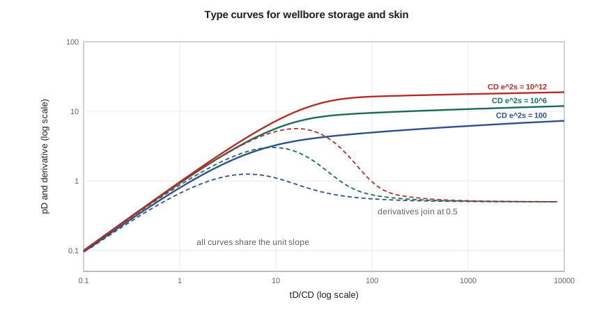
A type curve is a plot of a dimensionless solution, drawn so that a family of curves covers a range of a parameter. The standard storage-and-skin curves, published by Gringarten and colleagues in 1979, plot p_D against t_D/C_D on log-log axes for a range of values of the group C_D e^(2s). The insight behind this choice is that storage and skin act together: in the time window before radial flow, the response depends on C_D and s only through this combined group. Every curve starts on the same unit slope, where p_D = t_D/C_D, and bends over into radial flow at a point that depends on C_D e^(2s). High values of the group mean a damaged well with storage; low values mean a stimulated well.

Bourdet's derivative curves, added to the same plot in 1983, made the method far more reliable. Each derivative curve rises with the unit slope, passes through a hump whose height grows with C_D e^(2s), and settles on the radial-flow line at 0.5. The derivatives are easier to distinguish than the p_D curves, which crowd together near the bend.

Matching a test to a type curve

Type-curve matching works because the log-log plot of the field data has exactly the same shape as the dimensionless curve; it is only shifted. On log axes, multiplying a quantity by a constant moves the curve without changing its shape. The pressure change is p_D multiplied by a constant that contains kh, and the elapsed time is t_D/C_D multiplied by a constant that contains C, so the pressure shift reflects kh and the time shift reflects the storage coefficient. The engineer, or the software, slides the data over the type curves, holding the axes parallel, until the data and one curve coincide. A single match point, read from both grids, then gives the answers.

Here the subscript M marks the match point. The skin comes from the identified curve: s = 0.5 ln[(C_D e^(2s))_M / C_D], using C_D calculated from C. In metric units the constants change as before. Today, nonlinear regression adjusts the model parameters to minimize the misfit between model and data over the whole test, which is the computer equivalent of sliding the tracing paper. The regression is only as good as the model chosen, which is why the diagnostic step of lesson 5 comes first.

Type curves are also useful for planning. Before a test, an engineer can sketch the expected response from estimated parameters and see when radial flow should begin, how large the derivative hump will be, and whether a planned shut-in will reach the regime of interest. Lesson 12 uses this approach for the capstone design.

Partial penetration and limited entry

Many wells are open to only part of the formation, either because the lower part was left unperforated to delay water coning, or because only the best layer was perforated. Flow must then converge vertically toward the open interval, which adds a pressure drop called the partial-penetration skin. The total skin measured by a test combines this geometric skin with the damage skin. A well with zero damage but only a fifth of the zone open can show a measured skin of +5 or more, and acidizing it would not help.

On the diagnostic plot, partial penetration can show an early radial-flow period across the open interval, then a spherical or hemispherical flow period with a derivative slope of minus one half, then the full radial flow of the whole thickness. The spherical flow period, when it can be seen, gives the vertical permeability, which matters for coning studies and for horizontal wells. Separating geometric skin from damage skin requires the completion geometry and an estimate of the anisotropy ratio, and published correlations give the geometric skin for given penetration ratios and k_v/k_h.