
PET-360 · Lesson 5 of 12 · 16 min
The pressure derivative and diagnostic plots
When Ethan shows Rafael his semilog fits from lessons 3 and 4, Rafael asks only one question: 'How did you know where the straight line starts?' Ethan admits he picked the points that looked straight. Rafael opens the interpretation software, turns off every analysis plot, and leaves one window on the screen: a log-log plot of pressure change and something called the derivative. 'This is the first plot you make, every time,' he says. 'It tells you which model to use before you fit anything. Straight lines come afterwards.'
This lesson introduces the log-log diagnostic plot and the pressure derivative, shows how the derivative is computed from noisy field data, and describes the characteristic shapes, or signatures, that identify each flow regime. These signatures are the vocabulary of modern well test interpretation and are used in every remaining lesson.
The log-log plot
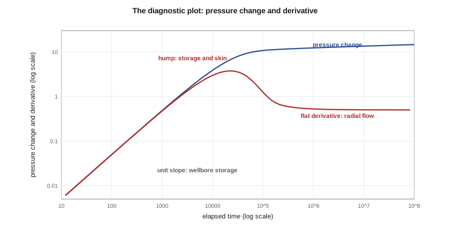
The simplest diagnostic plot shows the pressure change Δp against elapsed time Δt, both on logarithmic axes. For a drawdown, Δp = p_i − p_wf; for a buildup, Δp = p_ws − p_wf at shut-in. Log-log axes have a valuable property: if Δp is proportional to Δt raised to some power n, the data plot as a straight line with slope n. Several flow regimes produce exactly such power laws. Pure wellbore storage gives Δp proportional to Δt, a slope of one. Linear flow into a fracture gives a slope of one half. Bilinear flow gives a quarter. On the plain Δp curve, however, these slopes are hard to read, because a skin adds a constant that bends the curve, and radial flow, being logarithmic, has no fixed slope at all.
The pressure derivative
In 1983 Dominique Bourdet and colleagues proposed plotting, alongside Δp, the derivative of Δp with respect to the natural logarithm of time. Others had used time derivatives before, but the Bourdet form made them practical and is now standard.
The derivative has several remarkable properties. In radial flow, where Δp increases by m for each log cycle of time, the derivative is constant and equal to m/2.303, which is 70.6 qBμ/(kh) in oilfield units. A flat derivative is therefore the unmistakable signature of radial flow, and its level gives kh directly, with no straight-line picking on a semilog plot. Skin, being a constant, disappears from the derivative entirely. For power-law regimes, the derivative has the same slope as Δp and lies below it by a fixed ratio: for storage the two coincide, and for linear flow the derivative is exactly half of Δp. Changes in reservoir behaviour appear in the derivative long before they show clearly in Δp.
For a buildup, the time axis must account for the producing history. Analysts use either the superposition time function, which for a single prior rate reduces to the Horner time, or the equivalent time Δt_e = t_p Δt/(t_p + Δt), introduced by Agarwal in 1980. Using equivalent time, buildup data can be plotted on the same axes as a drawdown and compared with drawdown type curves, provided the producing time is not too short.
Computing the derivative from field data
Field pressures are recorded at irregular intervals and contain gauge noise. Differentiating noisy data amplifies the noise, so a naive point-to-point derivative is useless. The standard Bourdet algorithm uses, for each point, one neighbour on each side that is at least a chosen distance L away in the logarithm of time, and takes a weighted average of the two slopes. L is called the smoothing or differentiation interval and is typically 0.1 to 0.5 log cycles. Too small a value leaves the derivative noisy; too large a value smears real features such as the start of a boundary effect. A good practice is to try several values and check that interpreted features do not depend on the choice.
Other issues matter as much as the algorithm. The time of the rate change must be exact, because an error of a few minutes distorts all early data on a log scale. The reference pressure Δp is measured from must be correct; for a buildup it is the last flowing pressure before shut-in. Gauge drift, tidal effects in high-permeability reservoirs, and temperature changes in the wellbore can all create false features late in long tests. Rafael asks Ethan to plot the raw temperature from the gauge alongside every buildup, because a temperature step often explains a strange pressure wiggle.
# Pressure derivative: a drawdown with wellbore storage and skin, computed by Stehfest inversion
import math
SI = True
def I0(x):
    t = x / 3.75
    if x <= 3.75:
        y = t * t
        return 1 + y * (3.5156229 + y * (3.0899424 + y * (1.2067492 + y * (0.2659732 + y * (0.0360768 + y * 0.0045813)))))
    y = 1 / t
    return math.exp(x) / math.sqrt(x) * (0.39894228 + y * (0.01328592 + y * (0.00225319 + y * (-0.00157565 + y * (0.00916281 + y * (-0.02057706 + y * (0.02635537 + y * (-0.01647633 + y * 0.00392377))))))))
def I1(x):
    t = x / 3.75
    if x <= 3.75:
        y = t * t
        return x * (0.5 + y * (0.87890594 + y * (0.51498869 + y * (0.15084934 + y * (0.02658733 + y * (0.00301532 + y * 0.00032411))))))
    y = 1 / t
    return math.exp(x) / math.sqrt(x) * (0.39894228 + y * (-0.03988024 + y * (-0.00362018 + y * (0.00163801 + y * (-0.01031555 + y * (0.02282967 + y * (-0.02895312 + y * (0.01787654 - y * 0.00420059))))))))
def K0(x):                       # modified Bessel functions by polynomial approximations
    if x <= 2:
        y = x * x / 4
        return -math.log(x / 2) * I0(x) - 0.57721566 + y * (0.42278420 + y * (0.23069756 + y * (0.03488590 + y * (0.00262698 + y * (0.00010750 + y * 0.0000074)))))
    y = 2 / x
    return math.exp(-x) / math.sqrt(x) * (1.25331414 + y * (-0.07832358 + y * (0.02189568 + y * (-0.01062446 + y * (0.00587872 + y * (-0.00251540 + y * 0.00053208))))))
def K1(x):
    if x <= 2:
        y = x * x / 4
        return math.log(x / 2) * I1(x) + (1 / x) * (1 + y * (0.15443144 + y * (-0.67278579 + y * (-0.18156897 + y * (-0.01919402 + y * (-0.00110404 - y * 0.00004686))))))
    y = 2 / x
    return math.exp(-x) / math.sqrt(x) * (1.25331414 + y * (0.23498619 + y * (-0.03655620 + y * (0.01504268 + y * (-0.00780353 + y * (0.00325614 - y * 0.00068245))))))
def stehfest(F, t, N=12):         # numerical inversion of a Laplace-space function F(s) at time t
    ln2 = math.log(2); total = 0.0
    for i in range(1, N + 1):
        v = 0.0
        for k in range((i + 1) // 2, min(i, N // 2) + 1):
            v += k ** (N // 2) * math.factorial(2 * k) / (math.factorial(N // 2 - k) * math.factorial(k) * math.factorial(k - 1) * math.factorial(i - k) * math.factorial(2 * k - i))
        total += (-1) ** (i + N // 2) * v * F(i * ln2 / t)
    return total * ln2 / t

if SI:   # metric units: m3/d, m, kPa, mPa.s, 1/kPa, h
    q, B, mu, h, phi, ct, rw, k, s = 5.5, 1.29, 0.72, 6.5, 0.14, 1.5e-6, 0.089, 15.0, 5.0
    c_pD, c_tD, pu, CD = 1866.6, 3.553e-6, "kPa", 2000.0
else:    # field units: STB/d, ft, psi, cp, 1/psi, h
    q, B, mu, h, phi, ct, rw, k, s = 300.0, 1.25, 0.90, 30.0, 0.12, 1.2e-5, 0.35, 25.0, 5.0
    c_pD, c_tD, pu, CD = 141.2, 2.637e-4, "psi", 2000.0
def pD_lap(u):                         # Laplace-space solution: line source with storage CD and skin s
    r = math.sqrt(u)
    a = K0(r) + s * r * K1(r)
    return a / (u * (r * K1(r) + CD * u * a))
A = c_pD * q * B * mu / (k * h)
tD_per_h = c_tD * k / (phi * mu * ct * rw ** 2)
times = [0.01 * 1.6 ** i for i in range(22)]
dp = [A * stehfest(pD_lap, tD_per_h * t) for t in times]
def bourdet(i, L=0.25):                 # derivative with respect to ln t, using points at least L away
    x = [math.log(t) for t in times]
    j = i - 1
    while j > 0 and x[i] - x[j] < L: j -= 1
    m = i + 1
    while m < len(x) - 1 and x[m] - x[i] < L: m += 1
    d1 = (dp[i] - dp[j]) / (x[i] - x[j]); d2 = (dp[m] - dp[i]) / (x[m] - x[i])
    return (d1 * (x[m] - x[i]) + d2 * (x[i] - x[j])) / (x[m] - x[j])
print("   t (h)      dp        t*dp/dt")
for i in range(1, len(times) - 1, 2):
    print(f"{times[i]:8.3f}  {dp[i]:9.1f}  {bourdet(i):9.1f}")
flat = 0.5 * A
print(f"radial-flow plateau expected at {flat:.1f} {pu}; it gives kh = {c_pD * q * B * mu / (2 * flat):.0f}")t (h) dp t*dp/dt 0.016 34.1 34.4 0.041 84.5 82.4 0.105 200.8 179.4 0.268 432.8 313.5 0.687 766.1 341.0 1.759 1017.3 170.7 4.504 1111.7 68.9 11.529 1166.6 54.3 29.515 1215.6 50.8 75.558 1262.7 49.7 radial-flow plateau expected at 48.9 kPa; it gives kh = 98
The output shows the full sequence. The first points follow Δp almost exactly on a slope of one: storage. The derivative then rises to a hump near one hour and falls to a plateau that matches the predicted level within a few percent by about 30 hours; reading kh from that plateau gives the same answer as the semilog fits in lessons 3 and 4. The pressure change itself keeps rising slowly, as it must in radial flow.
Reading the signatures
Each part of the diagnostic plot corresponds to a region of the reservoir and a time in the test. Early time describes the wellbore and the near-well region: storage, skin, partial penetration and any hydraulic fracture. Middle time is the infinite-acting radial flow of the reservoir, where kh is measured. Late time describes the outer reservoir: faults, channels, closed boundaries, aquifers or gas caps. Some reservoirs add a middle-time feature of their own, such as the dip of a naturally fractured system.
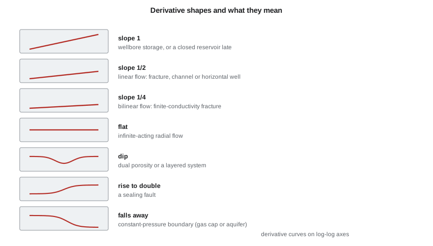
| Derivative shape | Likely cause | Lesson |
|---|---|---|
| Unit slope, merged with Δp | Wellbore storage | 6 |
| Hump after storage | Skin; a higher hump means a larger skin | 6 |
| Half slope, derivative at half of Δp | Linear flow: fracture, channel or horizontal well | 7, 9 |
| Quarter slope | Bilinear flow in a finite-conductivity fracture | 9 |
| Flat | Infinite-acting radial flow; level gives kh | 3 to 5 |
| Dip between two flat levels | Dual porosity or layered reservoir | 8 |
| Rise to twice the flat level | A single sealing fault | 7 |
| Late unit slope (drawdown) | Closed reservoir in pseudosteady state | 7 |
| Falling derivative | Constant-pressure boundary such as a gas cap or strong aquifer | 7 |
Non-uniqueness
The diagnostic plot is powerful, but it is not a magic key. Different reservoirs can produce the same shape. A late rising derivative might be a sealing fault, a change to lower permeability away from the well, or a closed boundary seen only partly in a buildup. A late falling derivative might be a constant-pressure boundary, or a change to higher permeability, or simply phase redistribution or gauge drift. The interpretation that wins is the one consistent with everything else known about the reservoir: seismic, geology, logs, production history and nearby tests. Rafael's rule is to write down every model that fits the shape, then discard those that conflict with independent data.
Another limitation is that buildups after short flow periods distort the late-time derivative. When the producing time is short, the shut-in response is dominated by the brief flow history, and the derivative can fall or rise at late time for no reason connected with the reservoir. Equivalent time partly corrects this, and deconvolution, introduced in lesson 12, addresses it more fully by combining all flow and shut-in periods into a single response.
Worked problem
Reading kh from the derivative plateau
A buildup on a Cardium well shows a flat derivative at 49 kPa. The rate before shut-in was 5.5 m³/d, B = 1.29 and μ = 0.72 mPa·s. What is kh?
Show solution
- In radial flow the derivative equals m/2.303, so m = 2.303 × 49 ≈ 113 kPa per cycle.
- In metric units, kh = 2,149 qBμ/m = 2,149 × 5.5 × 1.29 × 0.72/113 ≈ 97 mD·m.
- With h = 6.5 m, k ≈ 15 mD.
Answer: The derivative plateau gives the same kh as the semilog analysis, without having to choose points on a straight line by eye.
Common mistakes
MistakeFitting semilog lines before looking at the derivative.
InsteadMake the log-log diagnostic plot first and identify radial flow on it.
MistakeUsing too small a smoothing interval on noisy data.
InsteadTry several intervals; features should not depend on the choice.
MistakeUsing an inaccurate shut-in time.
InsteadGet the exact time of the rate change; early log-time data are very sensitive to it.
MistakeAccepting the first model that fits the shape.
InsteadList all models that fit and test them against geology and other data.
MistakeOver-reading late-time buildup derivatives after short flows.
InsteadUse equivalent or superposition time, or deconvolution, and treat late shapes with caution.
Summary and key terms
- The log-log plot shows power-law flow regimes as straight lines with characteristic slopes.
- The Bourdet derivative, dΔp/d ln Δt, is flat in radial flow at m/2.303, so its level gives kh and skin drops out.
- Storage gives a unit slope, linear flow a half slope and bilinear flow a quarter slope.
- Buildup derivatives use superposition or equivalent time to allow for the producing history.
- Derivatives of field data need smoothing over a log-time interval and exact rate-change times.
- Shapes are not unique; the chosen model must agree with geology and other data.
- Diagnostic plot
- A log-log plot of pressure change and derivative against elapsed time.
- Bourdet derivative
- The derivative of pressure change with respect to the natural logarithm of time.
- Flow regime
- A period during which flow has a characteristic geometry and pressure signature.
- Equivalent time
- Agarwal's time function t_p Δt/(t_p + Δt) for plotting buildups like drawdowns.
- Smoothing interval
- The log-time distance used to choose neighbouring points in the derivative calculation.
- Non-uniqueness
- The fact that different reservoir models can produce the same pressure response.
Practice problems
Work each problem on paper first, then reveal the answer to check.
What is the derivative's value in radial flow, in terms of m?
Show answer
m/2.303.
Why does skin not appear in the derivative?
Show answer
Skin adds a constant to Δp, and the derivative of a constant is zero.
What slope does linear flow show?
Show answer
One half, with the derivative at half of Δp.
What should you do when two models fit the derivative equally well?
Show answer
Use independent data such as seismic and geology to choose.
Lesson quiz · 5 questions
Score 60% or more to complete this lesson.
Create a free account to save your progress, take quizzes and earn a certificate.