Drawdown test analysis

The first test Ethan runs himself is a drawdown on the 100/08-27 delineation well, which was shut in for a week after its completion while the battery tie-in was finished. The pressure in the well is therefore uniform at the current pool pressure, about 14,090 kPa, which is the starting condition the theory needs. The pool's bubble point is near 12,800 kPa, so Rafael asks the operator to choke the well back to a steady 5.5 m³/d. 'If we pull the flowing pressure below the bubble point, gas comes out of solution near the well and our single-phase equations stop working,' he explains. 'A low rate with a clean signal beats a high rate with two phases.'

This lesson develops drawdown test analysis: the semilog method for permeability and skin, the effect of wellbore storage on early data, the radius of investigation as a check on what the test has sampled, and the reservoir limit test for closed systems. The same ideas carry over to buildups in lesson 4.

The semilog straight line

Lesson 2 showed that once wellbore effects have passed, the wellbore pressure in an infinite reservoir falls linearly with the logarithm of time. Writing the logarithmic approximation in oilfield units and in base-10 logarithms gives the working equation for a drawdown.

The slope m is the pressure change per log cycle of time, in psi per cycle for oilfield units. In the metric units used in Alberta, with the same symbols in kilopascals, cubic metres per day, metres and reciprocal kilopascals, the constant 162.6 becomes about 2,149 and the constant −3.23 becomes about −5.10. The equation says three things. First, a plot of p_wf against log t is a straight line with slope −m. Second, the slope gives kh directly: kh = 162.6 qBμ/m. Third, the position of the line, together with k, gives the skin.

This analysis is often called the MDH method, after the authors of an early paper on buildups, although for a drawdown it is simply the semilog form of the line-source solution. In practice the engineer plots the data, identifies the straight-line portion, fits a line through it, reads the slope, and reads the pressure on the line at a time of one hour, written p_1h. The skin follows by rearranging the equation at t = 1 h.

The value p_1h must be read from the straight line extended to one hour, not from the measured data at one hour. Early data are often still affected by wellbore storage, so the measured pressure at one hour may lie off the line. Reading from the line keeps the skin calculation consistent with the radial-flow model.

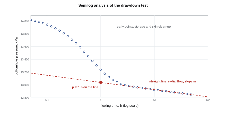
Picking the right straight line

The weakest step in semilog analysis is choosing which points lie on the straight line. Early in the test, wellbore storage and clean-up hold the pressure up, and a line drawn through those points gives a slope that is too small and a permeability that is too large. Late in the test, a boundary may bend the data. Before the diagnostic derivative plot became standard in the 1980s (lesson 5), engineers used rules of thumb such as waiting one and a half log cycles after the end of the unit-slope storage period. Today the derivative plot shows directly where radial flow is present, and the semilog line is fitted only through that period.

A useful habit is to calculate the slope from the fitted kh and check it against the derivative plateau, and to compute the radius of investigation at the start and end of the chosen period. If the straight line starts while the radius of investigation is still inside the damaged zone, or ends after the disturbance must have reached a known boundary, the choice is suspect.

# Drawdown test: semilog (MDH) analysis of a constant-rate flow period
import math
SI = True   
def E1(x):
    g, total, term = 0.5772156649, 0.0, 1.0
    for n in range(1, 60):
        term *= -x / n
        total += -term / n
    return -g - math.log(x) + total
if SI:   # metric units: m3/d, m, kPa, mPa.s, 1/kPa, h
    q, B, mu, h, phi, ct, rw, pi = 5.5, 1.29, 0.72, 6.5, 0.14, 1.5e-6, 0.089, 14090.0
    k_true, s_true = 15.0, 5.0
    c_m, c_pD, c_tD, c_log, pu = 2149.3, 1866.6, 3.553e-6, -5.10, "kPa"
else:    # field units: STB/d, ft, psi, cp, 1/psi, h
    q, B, mu, h, phi, ct, rw, pi = 300.0, 1.25, 0.90, 30.0, 0.12, 1.2e-5, 0.35, 3350.0
    k_true, s_true = 25.0, 5.0
    c_m, c_pD, c_tD, c_log, pu = 162.6, 141.2, 2.637e-4, -3.23, "psi"
def pwf(t):            # the "measured" pressure: line source plus skin, with a little gauge noise
    tD = c_tD * k_true * t / (phi * mu * ct * rw ** 2)
    pD = 0.5 * E1(1 / (4 * tD)) + s_true
    return pi - c_pD * q * B * mu / (k_true * h) * pD + 0.002 * pi * 0.01 * math.sin(7 * t)
times = [1, 2, 4, 8, 12, 16, 24, 36, 48]
data = [(t, pwf(t)) for t in times]
for t, p in data: print(f"t = {t:4.0f} h   pwf = {p:9.1f} {pu}")
pts = [(math.log10(t), p) for t, p in data if t >= 8]           # straight line after storage effects end
n = len(pts); sx = sum(x for x, _ in pts); sy = sum(y for _, y in pts)
sxx = sum(x * x for x, _ in pts); sxy = sum(x * y for x, y in pts)
slope = (n * sxy - sx * sy) / (n * sxx - sx * sx); icpt = (sy - slope * sx) / n
m = -slope                                      # pressure fall per log cycle
k = c_m * q * B * mu / (m * h)
p1h = icpt                                      # value of the straight line at t = 1 h
s = 1.1513 * ((pi - p1h) / m - math.log10(k / (phi * mu * ct * rw ** 2)) - c_log)
print(f"semilog slope m = {m:.1f} {pu} per log cycle")
print(f"permeability k = {k:.1f} mD   (kh = {k * h:.0f})")
print(f"p at 1 h on the line = {p1h:.1f} {pu}; skin s = {s:.2f}")
print(f"pressure drop across the skin = {0.869 * m * s:.0f} {pu}")

t =    1 h   pwf =   13038.3 kPa
t =    2 h   pwf =   13004.5 kPa
t =    4 h   pwf =   12970.4 kPa
t =    8 h   pwf =   12936.2 kPa
t =   12 h   pwf =   12916.8 kPa
t =   16 h   pwf =   12902.2 kPa
t =   24 h   pwf =   12882.4 kPa
t =   36 h   pwf =   12863.0 kPa
t =   48 h   pwf =   12848.8 kPa
semilog slope m = 112.4 kPa per log cycle
permeability k = 15.0 mD   (kh = 98)
p at 1 h on the line = 13037.8 kPa; skin s = 5.02
pressure drop across the skin = 491 kPa

Ethan's fit returns a permeability of 15 mD and a skin of about +5, with about 490 kPa of the drawdown lost across the damaged zone. The kh of about 98 mD·m is close to the core-weighted value from PET-350 and confirms that the Cardium here is the same rock as at the 102/06-14 well. The positive skin matches what Tom Ashworth suspected in PET-330: this well was perforated overbalanced, and the perforations are partly plugged.

What the skin means for production

The skin translates directly into lost production. The ideal productivity index with zero skin and the actual productivity index with skin s are related by the ratio of the logarithmic terms in the steady-state inflow equation from PET-320. A common summary is the flow efficiency: the ratio of the drawdown the well would need without skin to the drawdown it actually needs. With a skin of +5 in a well where the reservoir term ln(r_e/r_w) − 0.75 is about 7, the flow efficiency is about 7/12, or 58 percent. Removing the damage would raise the rate by roughly 70 percent at the same drawdown, which is the economic case for the acid treatments PET-330 designed.

Wellbore storage in a drawdown

When a well is opened at surface, the first fluid produced comes from expansion of the fluid already in the wellbore, not from the reservoir. The sandface rate starts at zero and climbs to the surface rate over minutes or hours. During that time the pressure response is controlled by the wellbore volume and fluid compressibility, and it carries no information about permeability. On a log-log plot of pressure change against time, pure storage gives a straight line of slope one, which lesson 5 uses to recognize it.

A rule of thumb for the end of storage effects, with C the wellbore storage coefficient in reservoir barrels per psi and the remaining quantities in oilfield units, is t ≈ (200,000 + 12,000 s) C/(kh/μ) hours. Large wellbores, gassy fluids and high skins all extend the storage period. Lesson 6 develops storage and its link with type curves.

The radius of investigation as a check

Every interpretation should end with a sanity check on how much rock the test has sampled. At the start of the straight line the radius of investigation should be well beyond the damaged zone, and at the end it shows how far the test has seen. For the 100/08-27 delineation well drawdown, the line starts at 8 hours, when the radius of investigation is already more than 100 m (400 ft), and ends at 48 hours at roughly 250 m (1,000 ft). A fault or pool edge beyond that distance would not yet affect the data.

The reservoir limit test

If a drawdown runs long enough for the disturbance to reach all the boundaries of a closed reservoir, flow changes from transient to pseudosteady state, as PET-320 lesson 10 introduced. In pseudosteady state, every point in the drainage area declines at the same rate, and the wellbore pressure falls linearly with time rather than with the logarithm of time.

Here A is the drainage area in square feet and the rate of decline is in psi per hour. A plot of p_wf against time on a linear scale becomes straight, and its slope gives the pore volume φhA connected to the well. This is the reservoir limit test, used to check whether a discovery is big enough to develop. It needs a long, steady drawdown, often weeks for a pool of useful size, and it is sensitive to rate changes, so it is usually run only when the answer is worth that effort. Modern rate-transient analysis (lesson 9) extracts the same information from routine production data with varying rates.

Drawdowns in practice: when the rate will not hold

Real drawdowns rarely deliver the perfectly steady rate the theory assumes. Separators surge, chokes erode, and a new well cleans up for days as completion fluids and fines come back. Two practical tools help. The first is to normalize the pressure by the rate: plotting (p_i − p_wf)/q against log t removes much of the effect of slow rate drift, because pressure drop is proportional to rate in a linear system. The second is to treat the test as a multirate test and use superposition explicitly, so that each recorded rate change contributes its own term. The superposition time function that results is plotted in place of log t, and the slope still gives kh. Modern software does this automatically, but the engineer must still supply a clean, correctly timed rate history, which is why Rafael insists on hourly rate readings for the whole test.

A related method is the two-rate test. Instead of shutting in, the operator changes the rate from one steady value to another and records the response. Production continues, so little oil is deferred, and because both rates are known the change in rate acts like a small buildup or drawdown that can be analysed with superposition. Two-rate tests suit wells that cannot be shut in, such as wells that load up with liquid when stopped, and they can also separate the rate-dependent part of the skin in gas wells (lesson 10).