
PET-360 · Lesson 12 of 12 · 18 min
Test design, interference testing and the capstone interpretation
Tom Ashworth's final request for the year is a test on the Tamarack 03-22 horizontal well before the company drills the Tamarack 04-22 horizontal well, planned 200 m away. The question is simple to ask and hard to answer: will the new well drain new rock, or will it share rock that the 03-22 already drains? If the two wells interfere strongly, the spacing for the whole western development should widen, which changes the number of wells by a third. Ethan now has to put everything from the course together: what to measure, how long to test, what the data could show, and how sure anyone can be.
This capstone lesson covers the design of a well test from its objective backwards, the use of multiwell interference and pulse tests, deconvolution of multi-rate data, quality control and the structure of a good interpretation report. It ends with the design and expected response of the 03-22 buildup.
Design starts with the question
Every test should begin with a written objective that names the decision it supports. 'Measure the permeability' is not an objective; 'decide whether a second well 200 m away will drain new rock' is. The objective determines which flow regime must be reached, and the flow regime determines the duration, the rate, the gauge requirements and the cost. A useful design sequence is: state the decision; identify the reservoir property or feature that controls it; find the flow regime in which that property shows on the derivative; estimate when the regime starts and ends using the radius of investigation and the type curves of lessons 5 to 9; and check whether the expected pressure change is large enough to measure.
Design also has to consider the cost of the test itself. A shut-in defers production, a drawdown may need a flare permit or a pipeline connection, and a downhole gauge run may require a wireline unit or a workover. The value of the information, compared with the cost of the decision it supports, decides whether the test is worth doing. In many cases a planned shut-in for some other reason, such as a facility turnaround, gives a free buildup if a gauge is in place.
Gauges and data quality
Modern quartz pressure gauges resolve changes of less than 0.01 psi (about 0.07 kPa) and are stable over weeks. Strain gauges are cheaper and less precise. Resolution matters most late in a test, where the derivative is computed from small pressure changes, and in interference tests, where the signal at the observation well may be only a few kilopascals or psi. Gauge drift, a slow change in reading unrelated to pressure, can mimic a boundary in a long test, so two gauges in tandem are standard for important tests. Temperature should always be recorded with pressure, and the clock must be synchronized with the rate records, because a mistake of a few minutes in the shut-in time distorts the early derivative.
Before interpreting, the analyst checks the data. Are the pressures and rates consistent with the wellbore hydraulics? Is the shut-in time exact? Do the two gauges agree? Do pressure jumps coincide with operational events in the daily reports? Is there evidence of phase redistribution, leaks or tidal effects? Only after these checks does the diagnostic plot become meaningful.
Interference and pulse tests
In an interference test, one well, the active well, changes its rate, and the pressure is recorded at a separate observation well. The response at the observation well depends on the reservoir between the wells. For a homogeneous reservoir, the line-source solution of lesson 2 applies directly with r equal to the well spacing, and type-curve matching of the observation-well response gives kh and the storativity φc_t h between the wells. Interference tests answer questions no single-well test can: whether two wells are connected, how fast pressure moves between them, and whether the connection is directional, which several observation wells can reveal.
The difficulty is the small signal. Pressure changes at an observation well hundreds of metres away may be a few kilopascals, and they arrive after a delay. A pulse test, introduced by Johnson, Greenkorn and Woods in the 1960s, alternates the active well between flow and shut-in in short pulses. The observation well sees a small periodic signal that can be separated from background trends, and the lag and amplitude of the pulses give the reservoir properties. Pulse tests are shorter than interference tests and less sensitive to drift.
Deconvolution
Real tests seldom have a single clean rate change. A drawdown is often followed by a buildup, then another flow, then another shut-in. Each period on its own shows only a short part of the reservoir response. Deconvolution, made practical by the work of von Schroeter, Hollaender and Gringarten and of Levitan in the early 2000s, combines all the pressure and rate data into a single equivalent constant-rate drawdown response lasting as long as the whole test. A buildup of 100 hours after six months of production can therefore show the reservoir response out to six months, and boundaries invisible in any single period may appear. The method needs accurate rate histories and consistent pressures, and its late-time results should be checked by testing whether different subsets of the data give the same answer.
The capstone design
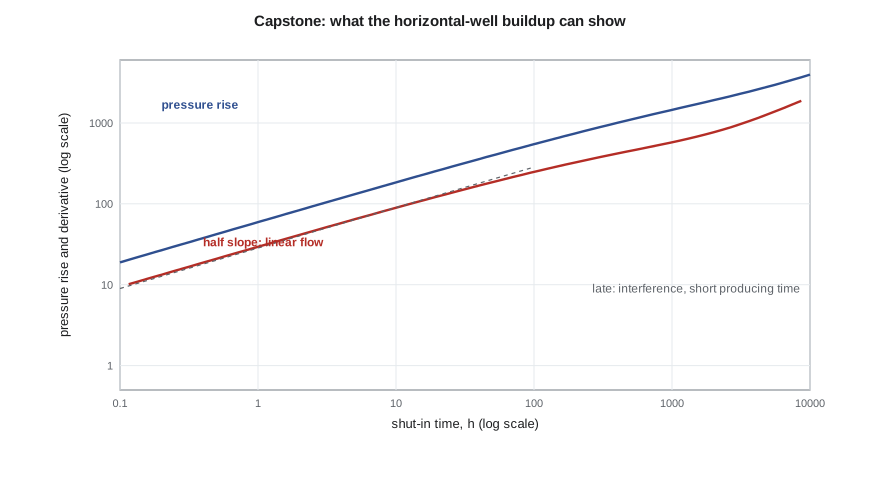
The 03-22 has produced 120 days at about 40 m³/d. A buildup is the obvious test, and a pressure gauge can be set above the packer on the next pump change. Ethan uses the linear-flow model from lesson 9 and the flow area and permeability from the RTA to predict the buildup response, then asks two questions: how long until the transient reaches halfway to the 04-22 location, which is when interference between the two would begin to show; and whether the late pressure changes would be measurable.
# Capstone: design and interpret a buildup on the new horizontal well, which stays in linear flow
import math
SI = True
DAY, HR, MD = 86400.0, 3600.0, 9.869e-16
if SI:
    q_si, B, mu_cp, phi, ct_kpa, h = 40.0 / DAY, 1.29, 0.72, 0.14, 1.5e-6, 6.5   # 40 m3/d before shut-in
    n_frac, xf, k_md = 40, 30.0, 0.5
    ct, tp = ct_kpa / 1e3, 120 * DAY
    pfac, pu, du, gauge = 1e-3, "kPa", "m", 0.07                                 # gauge resolution in kPa
else:
    q_si, B, mu_cp, phi, ct_psi, h = 600 * 0.158987 / DAY, 1.456, 0.40, 0.08, 1.5e-5, 45.0 * 0.3048
    n_frac, xf, k_md = 60, 250.0 * 0.3048, 0.005
    ct, tp = ct_psi / 6894.76, 120 * DAY
    pfac, pu, du, gauge = 1 / 6894.76, "psi", "ft", 0.01
mu, k = mu_cp * 1e-3, k_md * MD
Ac = n_frac * 2 * xf * h; eta = k / (phi * mu * ct)
mL = 2 * B * mu * q_si / (k * Ac) * math.sqrt(eta / math.pi)        # Pa per sqrt(s): drawdown = mL sqrt(t)
def rise(dt):                                                       # superposition for a linear-flow buildup
    return mL * (math.sqrt(tp) + math.sqrt(dt) - math.sqrt(tp + dt))
print("  shut-in (h)   pressure rise     log-log slope")
prev = None
for hrs in (1, 3, 10, 30, 100, 300, 700):
    dt = hrs * HR; r = rise(dt) * pfac
    sl = math.log(rise(dt * 1.1) / rise(dt / 1.1)) / math.log(1.21)
    print(f"{hrs:10d}   {r:12.1f} {pu}   {sl:8.2f}")
half_gap = (100.0 if SI else 330.0 * 0.3048)                        # half the distance to the neighbouring well
t_bound = half_gap ** 2 / (4 * eta)                                 # rough diffusion time across that distance
print(f"rough time for the transient to reach midway to the neighbouring well: {t_bound / HR:.0f} h ({t_bound / DAY:.0f} days)")
late = (rise(700 * HR) - rise(300 * HR)) * pfac
print(f"pressure change between 300 and 700 h: {late:.0f} {pu}, far above the gauge resolution of {gauge} {pu}")
print("the slope falls below 0.5 because the well produced for only 120 days; use superposition time to correct it") shut-in (h) pressure rise log-log slope
1 214.0 kPa 0.50
3 368.2 kPa 0.49
10 663.1 kPa 0.48
30 1123.1 kPa 0.47
100 1960.9 kPa 0.45
300 3153.2 kPa 0.41
700 4383.6 kPa 0.36
rough time for the transient to reach midway to the neighbouring well: 213 h (9 days)
pressure change between 300 and 700 h: 1230 kPa, far above the gauge resolution of 0.07 kPa
the slope falls below 0.5 because the well produced for only 120 days; use superposition time to correct itThe prediction is encouraging. The pressure rise follows a half slope at first, and the time for the transient to reach midway to the 04-22 location is about 213 hours, or 9 days. A shut-in of four weeks would therefore see beyond the midpoint, and the pressure change between 300 and 700 hours is about 1,230 kPa, enormously larger than the gauge resolution. The late bend of the derivative below the half slope is caused by the short producing time, not by the reservoir, so the interpretation will use superposition time and deconvolution with the full production history. Ethan recommends a 28-day buildup, with production deferred during it, and an interference check when the 04-22 is completed.
Integrating the interpretation
A well test interpretation is a model, and it should agree with everything else known about the reservoir. The permeability-thickness should be consistent with core and log permeabilities, allowing for scale differences. Boundary distances should match seismic and geology. The skin should fit the completion history. The p* or average pressure should agree with material balance. When the test disagrees with other data, the disagreement is information: it may show that the core is unrepresentative, that a fault mapped as sealing is not, or that the test model is wrong.
A good interpretation report states the objective, the test sequence with rates and times, the data quality checks, the diagnostic plot with the flow regimes identified, the model chosen and the alternatives considered, the parameters with uncertainty ranges, the consistency checks against other data, and the answer to the original question. A one-page summary at the front gives the decision-maker the answer; the rest lets another engineer check the work. Uncertainty ranges should come from how far the parameters can change while still matching the data, and from the spread between alternative models, not from regression statistics alone.
| Step | Key questions | Lesson |
|---|---|---|
| Objective | Which decision? Which property controls it? | 1 |
| Flow regime | Where does that property appear on the derivative? | 5 to 9 |
| Duration | When does the regime start and end? Radius of investigation? | 6, 7 |
| Measurement | Is the signal larger than gauge resolution and noise? | 12 |
| Data checks | Exact times, consistent gauges, events explained? | 5, 12 |
| Interpretation | Diagnose, choose models, match, compare alternatives | 5 to 11 |
| Integration | Consistent with core, logs, seismic and material balance? | 12 |
| Report | Answer the question with uncertainty ranges | 12 |
Worked problem
Will a buildup see the boundary?
A vertical Cardium well in 15 mD rock (φ = 0.14, μ = 0.72 mPa·s, c_t = 1.5 × 10⁻⁶ kPa⁻¹) is suspected to lie 300 m from a sealing fault. The planned buildup is 72 hours. Will it see the fault?
Show solution
- The radius of investigation at 72 hours is √(15 × 72/(70,350 × 0.14 × 0.72 × 1.5 × 10⁻⁶)) ≈ 318 m.
- That is about the fault distance, but a clear fault signature needs r_i of two to three times the distance.
- The test would need roughly four to eight times longer, 11 to 24 days, assuming the flow before it was at least as long.
Answer: A 72-hour buildup would show at most the very start of the fault effect. Either extend the test, or accept that it answers a different question, such as kh and skin.
Common mistakes
MistakeDesigning a test without a written objective.
InsteadName the decision and the flow regime needed before choosing the duration.
MistakeAssuming the shut-in alone sets what a buildup can see.
InsteadThe flow period before it also limits the response; use deconvolution for long histories.
MistakeUsing a single gauge on a critical test.
InsteadRun two gauges in tandem and record temperature.
MistakeReporting a single answer without alternatives.
InsteadShow the alternative models and the uncertainty ranges.
MistakeIgnoring disagreement with core, logs or seismic.
InsteadTreat disagreement as information and explain it.
Summary and key terms
- Design starts with the decision, then the property, the flow regime, the duration and the measurement.
- Quartz gauges, tandem gauges, temperature and exact times are essential for good data.
- Interference and pulse tests measure connectivity and properties between wells.
- Deconvolution combines all rate periods into one long equivalent drawdown.
- Short producing times distort late buildup derivatives; superposition time and deconvolution correct for it.
- A good report answers the question with alternatives, uncertainty and consistency checks.
- Test objective
- A statement of the decision a test supports and the property it must measure.
- Interference test
- A test in which pressure is recorded at an observation well while an active well changes rate.
- Pulse test
- An interference test using alternating short flow and shut-in periods.
- Deconvolution
- A method that converts a multi-rate test into an equivalent constant-rate drawdown response.
- Gauge resolution
- The smallest pressure change a gauge can detect.
- Gauge drift
- A slow change in gauge reading not caused by pressure.
Practice problems
Work each problem on paper first, then reveal the answer to check.
What should a test objective name?
Show answer
The decision the test supports.
What does an interference test measure that a single-well test cannot?
Show answer
Connectivity and properties between wells.
What does deconvolution produce?
Show answer
An equivalent constant-rate drawdown lasting the whole test.
Why record temperature with pressure?
Show answer
Temperature changes can explain pressure anomalies and gauge effects.
Lesson quiz · 5 questions
Score 60% or more to complete this lesson.
Create a free account to save your progress, take quizzes and earn a certificate.