Gas well testing and deliverability

Prairie Crest has bought a small interest in the Birch Coulee gas pool, and the operator has sent over the results of a new deliverability test on the 100/10-09 gas well: four short flow periods at increasing rates, each followed by a shut-in, and one long final flow. The partner's report gives an absolute open flow of about 600 thousand cubic metres per day. Tom Ashworth wants to know whether to believe it before the company commits to its share of a new compressor. Ethan has never analysed a gas test, and finds that almost everything he has learned still applies, with two important changes.

This lesson covers the two differences between gas and liquid tests, the pressure dependence of gas properties and non-Darcy flow, and then the deliverability tests used to predict how much a gas well can produce against a given back pressure: flow-after-flow, isochronal and modified isochronal tests, analysed by the back-pressure equation and by the laminar-inertial-turbulent (LIT) method.

Pseudo-pressure

The diffusivity equation of lesson 2 assumed a slightly compressible liquid with constant viscosity. Gas is highly compressible, and its viscosity and z-factor change strongly with pressure, so the equation becomes nonlinear. In 1966 Al-Hussainy, Ramey and Crawford showed that it can be made nearly linear again by replacing pressure with the real-gas pseudo-pressure:

In terms of m(p), the gas flow equation has the same form as the liquid equation, and all the solutions of earlier lessons, including the semilog line, the derivative and the type curves, apply with m(p) in place of p. The remaining nonlinearity is in the product μc_t in the diffusivity, which still changes with pressure; for drawdowns with large pressure changes, analysts also use pseudo-time, which integrates 1/(μc_t) over time.

Two simpler approximations follow from the shape of p/(μz). At low pressures, below roughly 14,000 kPa or 2,000 psi, μz is nearly constant, so m(p) is proportional to p², and the pressure-squared form of the equations is adequate. At high pressures, above roughly 21,000 kPa or 3,000 psi, p/(μz) is nearly constant, so m(p) is proportional to p, and the liquid equations can be used directly with gas properties at the average pressure. Between those ranges, and whenever the drawdown is large, pseudo-pressure is the safe choice. Modern software calculates it routinely from the gas composition.

In oilfield units, the semilog slope for a gas well in pseudo-pressure terms is m = 1,637 q T/(kh), where q is in Mscf/d, T in degrees Rankine and m(p) in psi² per cP. The temperature enters because the rate is measured at surface conditions and the gas expands in the reservoir as it heats up. The metric constant differs, as always.

Non-Darcy flow and rate-dependent skin

Darcy's law assumes that flow is slow enough that friction is the only resistance. Near a gas well, velocities are high, and inertia, the energy lost as gas accelerates and decelerates through pore throats, adds a second resistance. Forchheimer described it in 1901 as a term proportional to the velocity squared. In well testing, the effect appears as an extra skin that increases with rate:

Here s' is the apparent skin measured by a test, s is the true mechanical skin and D is the non-Darcy coefficient. Because the extra pressure drop is concentrated close to the well where velocities are highest, it acts like a skin. To separate s from D, the well must be tested at two or more rates: a plot of s' against q is a straight line with intercept s and slope D. A gas well tested at a single rate, reporting a skin of +6, could be a damaged well or a perfectly clean well with high turbulence; acid would help the first and do nothing for the second.

Deliverability tests

Deliverability is the relation between the gas rate and the bottomhole flowing pressure under stabilized conditions. Its classic summary is the absolute open flow potential (AOF), the theoretical rate if the bottomhole pressure were reduced to atmospheric. No well produces at its AOF, but regulators and partners use it as a standard measure, and the full deliverability curve is what facility design needs.

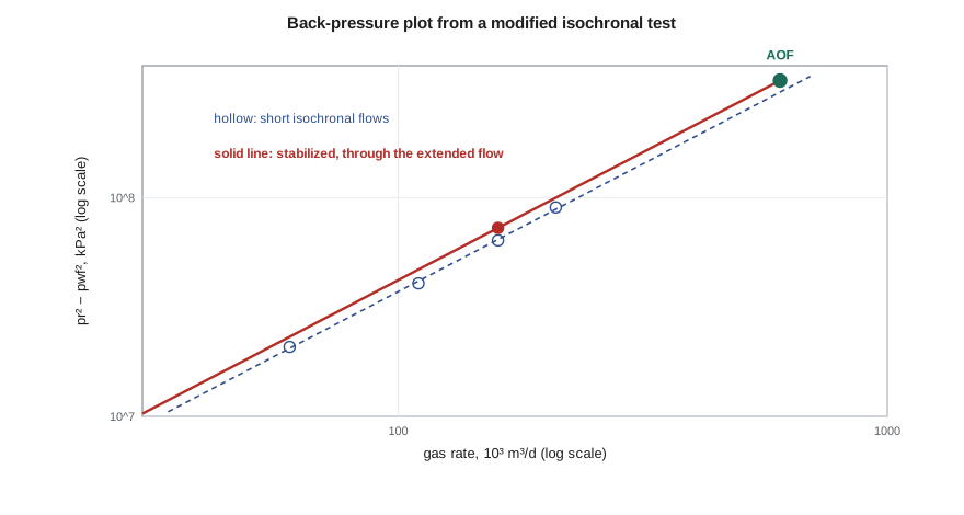
The oldest test is the flow-after-flow or back-pressure test, published by Rawlins and Schellhardt of the U.S. Bureau of Mines in 1936. The well flows at three or four rates in sequence, each until the pressure stabilizes. In high-permeability gas reservoirs, stabilization takes hours; in tight gas, it can take weeks or longer, so a stabilized multi-rate test is impractical. Cullender proposed the isochronal test in 1955. Each flow period lasts the same short time and is followed by a shut-in long enough for the pressure to return to the reservoir pressure; flows of equal duration probe the same radius, so their points line up on a curve parallel to the stabilized one. One long extended flow gives a single stabilized point, through which the stabilized curve is drawn. The modified isochronal test shortens the shut-ins to the same length as the flows, which saves time and is accurate enough in most reservoirs.

The back-pressure equation

Rawlins and Schellhardt found empirically that the stabilized rate follows a simple power law of the pressure-squared difference:

On a log-log plot of (p̄_R² − p_wf²) against q, the points form a straight line with slope 1/n. The exponent n is between 0.5 and 1: a value of 1 means purely laminar Darcy flow, and a value approaching 0.5 means that non-Darcy losses dominate. The coefficient C depends on the flow period, so the isochronal points give n, and the extended flow fixes C for stabilized conditions. Substituting atmospheric pressure for p_wf gives the AOF.

The LIT method

The back-pressure equation is empirical, and its exponent can drift if extrapolated far beyond the test rates. A more physical form, associated with Houpeurt, writes the pressure-squared or pseudo-pressure difference as a laminar term plus a turbulent term:

Dividing by q gives a straight line on a Cartesian plot of (p̄_R² − p_wf²)/q against q, with intercept a and slope b. The coefficient a contains kh, skin and the drainage geometry; b contains the non-Darcy coefficient. Solving the quadratic for q at any flowing pressure gives the deliverability, and the AOF follows from p_wf at atmospheric pressure. The LIT form is preferred for extrapolation and when the test pressures are high enough that pseudo-pressure should replace p².

# Gas well deliverability: a modified isochronal test, the back-pressure equation and the AOF
import math
SI = True   
if SI:   # metric: kPa, 10^3 m3/d
    pr, patm, pu, qu = 18500.0, 101.3, "kPa", "10^3 m3/d"
    tests = [(60.0, 17930.0), (110.0, 17370.0), (160.0, 16690.0), (210.0, 15880.0)]   # rate, flowing pressure
    extended = (160.0, 16420.0)          # the long final flow period, read at stabilized time
else:    # field: psia, Mscf/d
    pr, patm, pu, qu = 2680.0, 14.7, "psia", "Mscf/d"
    tests = [(2100.0, 2597.0), (3900.0, 2516.0), (5600.0, 2418.0), (7400.0, 2300.0)]
    extended = (5600.0, 2378.0)
print(" rate          pwf      pr^2 - pwf^2")
pts = []
for q, p in tests:
    d = pr ** 2 - p ** 2; pts.append((math.log10(q), math.log10(d)))
    print(f"{q:7.0f} {qu}  {p:7.0f}  {d:12.4g}")
n_pts = len(pts); sx = sum(x for x, _ in pts); sy = sum(y for _, y in pts)
sxx = sum(x * x for x, _ in pts); sxy = sum(x * y for x, y in pts)
b = (n_pts * sxy - sx * sy) / (n_pts * sxx - sx * sx)      # slope of log(dp2) against log(q) = 1/n
n = 1 / b
q_ext, p_ext = extended
C = q_ext / (pr ** 2 - p_ext ** 2) ** n                     # stabilized line through the extended point
aof = C * (pr ** 2 - patm ** 2) ** n
print(f"back-pressure exponent n = {n:.3f} (1 for laminar flow, 0.5 for fully turbulent)")
print(f"stabilized coefficient C = {C:.4g}  (q = C (pr^2 - pwf^2)^n)")
print(f"absolute open flow potential = {aof:.0f} {qu}")
# the same data as a laminar-inertial (LIT) fit: dp2 = a q + b q^2
xs = [q for q, _ in tests]; ys = [(pr ** 2 - p ** 2) / q for q, p in tests]
mx = sum(xs) / len(xs); my = sum(ys) / len(ys)
bb = sum((x - mx) * (y - my) for x, y in zip(xs, ys)) / sum((x - mx) ** 2 for x in xs); aa = my - bb * mx
print(f"LIT form: dp2/q = {aa:.4g} + {bb:.4g} q  (the second term is the non-Darcy part)")

 rate          pwf      pr^2 - pwf^2
     60 10^3 m3/d    17930     2.077e+07
    110 10^3 m3/d    17370     4.053e+07
    160 10^3 m3/d    16690     6.369e+07
    210 10^3 m3/d    15880     9.008e+07
back-pressure exponent n = 0.856 (1 for laminar flow, 0.5 for fully turbulent)
stabilized coefficient C = 2.958e-05  (q = C (pr^2 - pwf^2)^n)
absolute open flow potential = 604 10^3 m3/d
LIT form: dp2/q = 3.103e+05 + 556.3 q  (the second term is the non-Darcy part)

The four flows give an exponent of 0.86, indicating a modest non-Darcy contribution. With the stabilized coefficient from the extended flow at 160 thousand cubic metres per day, the AOF is about 604 × 10³ m³/d, close to the partner's figure. The LIT fit gives a = 3.10 × 10⁵ and b = 556 in kPa² per unit rate; at the highest test rate, the turbulent term is about 27 percent of the total drawdown. Ethan concludes that the number is credible, but that the well's deliverability at the planned compressor suction pressure, not the AOF, is what the decision needs.

Gas test practicalities

Gas tests bring their own hazards and data problems. Liquid loading in low-rate wells can make the flowing pressure erratic. Condensate dropout below the dew point forms a liquid bank near the well in gas-condensate reservoirs, which shows up as a composite-like response and an extra skin that depends on rate and time. Hydrates can form in the test equipment if water is present and temperatures fall. Flaring during a test is regulated, and in many jurisdictions the flared volume and the duration of the test are limited, which shapes the test design. Directive 040 sets out testing requirements for gas wells, and partners usually specify the deliverability test method in operating agreements.

Gas buildups and drill-stem tests in gas zones

A buildup on a gas well is analysed like an oil buildup once pseudo-pressure replaces pressure. The Horner or superposition plot of m(p) gives kh from the slope, and the skin from the plot is the apparent skin s' at the rate before shut-in. If two buildups follow flows at different rates, the two apparent skins give s and D, as in the multi-rate plot described above. Wellbore storage is usually larger in gas wells because gas is so compressible, so downhole shut-in matters even more than for oil.

Gas zones are often first tested with a drill-stem test, before the well is cased. A DST tool string isolates the zone with packers, opens it to the drill pipe for a short flow, then closes a downhole valve for a buildup, usually repeating the cycle twice. The short initial flow relieves any supercharging of the near-well rock by drilling mud filtrate, and the first buildup gives a reliable initial reservoir pressure. The second, longer flow and buildup give kh and skin. Because the flows are short, DST buildups see only a small radius, but they are often the only test before the decision to complete or abandon the well.

Gas-condensate reservoirs need extra care. If the flowing pressure falls below the dew point, liquid condenses near the well and reduces the gas relative permeability, creating a ring of lower mobility. The derivative then shows a radial composite response, and the apparent skin rises with drawdown. Testing condensate wells at modest drawdowns, and sampling the fluid early while the reservoir is still above the dew point, avoids misleading results.