Pulse processing electronics

Every detector in this course produces, at its output, a small and brief burst of charge. Between that burst and the number in a database sits a chain of electronics that most users never think about, until something goes wrong. One afternoon the germanium detector Hana relies on starts producing broad, lopsided peaks. The detector is fine; a shaping amplifier setting was changed for a high-rate measurement and never set back. Marcel uses the incident to teach her what each box in the chain does and how its settings change the result.

The signal chain

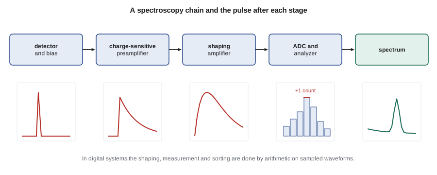
A typical spectroscopy chain has five stages. The detector bias supply provides the field that collects charge. The preamplifier, mounted close to the detector, converts the collected charge into a voltage step. The shaping amplifier filters and amplifies that step into a pulse whose height is proportional to the charge and whose shape optimizes the ratio of signal to noise. An analogue-to-digital converter measures the pulse height. A multichannel analyzer sorts the measured heights into a histogram, the spectrum. In modern digital systems, the last three stages are combined: the preamplifier output is sampled at high speed and the shaping, height measurement and sorting are done by arithmetic in a field-programmable gate array.

Counting systems that do not need energy information, such as GM survey meters or gross alpha-beta counters, replace the analyzer with discriminators and scalers. A discriminator produces a logic pulse whenever the input exceeds a set threshold. A single-channel analyzer produces one only when the pulse falls between a lower and an upper threshold, defining a window. A scaler counts the logic pulses and a timer sets the counting interval. A ratemeter averages pulses over a time constant to display a count rate, as on a survey meter's dial.

Preamplifiers

A charge-sensitive preamplifier integrates the detector current on a small feedback capacitor \(C_f\). Its output step has height \(V = Q/C_f\), independent of the detector's own capacitance, which changes with bias and temperature. A feedback resistor slowly discharges the capacitor so that the output returns to baseline with a time constant of tens to hundreds of microseconds. Some germanium preamplifiers instead reset the capacitor periodically with a transistor switch, which lets them handle very high count rates.

The preamplifier is where most of the electronic noise originates, so it is placed as close to the detector as possible and, for germanium, its input transistor is often cooled along with the crystal. Long cables between detector and preamplifier add capacitance and noise and pick up interference, which is why preamplifiers sit on the detector housing. Microphonics, the noise from mechanical vibration changing capacitances, is another preamplifier problem and the reason detectors are not placed near pumps or heavy doors.

Shaping amplifiers

The preamplifier output is a step with a long tail, unsuitable for measurement at any useful count rate because successive steps would pile on each other. The shaping amplifier turns each step into a short pulse. The classic design passes the signal through a differentiator (a CR filter), which removes the long tail, and one or more integrators (RC filters), which smooth high-frequency noise. A CR-RC shaper with time constant \(\tau\) gives a unipolar pulse

that peaks at \(t = \tau\). Real amplifiers use several integrators to give a nearly Gaussian shape, and pole-zero cancellation to remove the undershoot that a differentiator would otherwise produce from the preamplifier's exponential tail. Incorrect pole-zero adjustment is one of the most common causes of degraded resolution at high rates, because each pulse sits on the undershoot of the one before.

# Pulse processing: CR-RC shaping, pile-up probability and dead-time models.
import math
tau = 1.0                       # shaping time constant, microseconds
peak_t = tau                    # CR-RC pulse peaks at t = tau
print("CR-RC pulse (normalized): t/tau, height")
for t in (0.25, 0.5, 1.0, 2.0, 3.0, 5.0):
    v = (t / tau) * math.exp(1 - t / tau)
    print(f"  {t:4.2f}  {v:5.3f}")

# Pile-up: probability another pulse arrives within resolving time T of a given pulse
T = 6e-6
for rate in (1e3, 1e4, 5e4, 1e5):
    p = 1 - math.exp(-2 * rate * T)
    print(f"rate {rate:8.0f} cps: pile-up fraction {100*p:5.2f} %")

# Dead time: true rate n from measured m, both models, tau_d = 20 microseconds
td = 20e-6
print("\nmeasured, non-paralyzable true, paralyzable true")
for m in (1000, 5000, 15000):
    n_np = m / (1 - m * td)
    n = m                         # solve m = n exp(-n td) by iteration (low-rate branch)
    for _ in range(60): n = m * math.exp(n * td)
    print(f"{m:6d}  {n_np:8.0f}  {n:8.0f}")

CR-RC pulse (normalized): t/tau, height
  0.25  0.529
  0.50  0.824
  1.00  1.000
  2.00  0.736
  3.00  0.406
  5.00  0.092
rate     1000 cps: pile-up fraction  1.19 %
rate    10000 cps: pile-up fraction 11.31 %
rate    50000 cps: pile-up fraction 45.12 %
rate   100000 cps: pile-up fraction 69.88 %

measured, non-paralyzable true, paralyzable true
  1000      1020      1021
  5000      5556      5592
 15000     21429     24470

The shaping time is a compromise. Longer shaping averages over more noise and integrates the charge fully even when it is collected slowly, giving the best resolution at low count rates. Shorter shaping makes pulses narrower, so more can be processed per second with less pile-up, but it lets in more noise and can lose charge from slowly collected events, the ballistic deficit described in lesson 4. Germanium systems for environmental samples typically use shaping times of about 4 to 6 µs; for high-rate reactor samples, 1 to 2 µs may be chosen. The setting Hana found had been reduced to 0.5 µs, and the broad, tailed peaks were the result.

Pulse height analysis

The multichannel analyzer divides the range of pulse heights into channels, typically 4096 to 16 384 for germanium spectroscopy and 1024 for NaI. Each pulse adds one count to the channel matching its height. Two properties of the ADC matter. Its integral linearity determines how accurately channel number follows energy, which affects identification. Its differential linearity determines how evenly the channel widths are spaced; poor differential linearity creates small artificial ripples in the spectrum. Modern ADCs and digital processors are very good on both counts, and the remaining nonlinearity is absorbed into the energy calibration.

Gain and zero drift are slower problems. Temperature changes in the preamplifier, amplifier or high voltage supply move peaks across channels over hours, which broadens peaks in long counts. Digital stabilizers lock on to a reference peak and correct the gain automatically. The daily check-source measurement in lesson 11 records peak position and width so that drift is noticed.

Pile-up

If a second pulse arrives before the first has been measured, the two can combine into a single pulse of wrong height. Pile-up removes counts from the photopeak and adds them at higher energies, distorting both. For random arrivals at rate \(r\) and a resolving time \(T\), the fraction of events affected is about

The program shows that with a 6 µs resolving time, pile-up affects about 1 % of events at 1000 counts per second but more than 10 % at 10 000. Pile-up rejection circuits use a fast parallel channel to detect a second pulse during the processing of the first and discard both. The rejection loses counts, so the live-time correction must account for it, which modern analyzers do.

Dead time

Every counting system has a minimum time after an event during which it cannot record another. Two idealized models describe the behaviour. In a non-paralyzable system, events that arrive during the dead time are simply lost, but they do not extend it. If \(m\) is the measured rate, \(n\) the true rate and \(\tau\) the dead time,

In a paralyzable system, each event, recorded or not, restarts the dead time. The measured rate is then

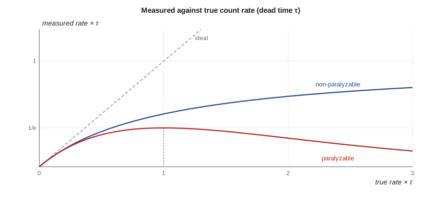
At low rates the two models agree, but they diverge at high rates. A non-paralyzable counter's measured rate approaches \(1/\tau\) and stays there. A paralyzable counter's measured rate reaches a maximum of \(1/(e\tau)\) at a true rate of \(1/\tau\) and then falls, so a very high true rate can give a low reading. This is the physics behind GM survey meters reading low in very high fields, noted in lesson 2. Real systems are often a mix, and the dead time of a counting system can be measured with the two-source method in lesson 12.

For spectroscopy, analyzers correct for dead time automatically by measuring live time: the clock that counts real time is gated off while the system is busy. That works well when the count rate is steady during the measurement. When the rate changes quickly, as with short-lived radionuclides counted soon after a sample is taken, live-time correction can be biased, and techniques such as loss-free counting, which adds a weighted count for each one lost, are used instead.

Coincidence and timing circuits

Some measurements depend on the timing between pulses rather than their heights. A coincidence circuit produces an output only when two detectors fire within a short window, a few nanoseconds to a microsecond. Coincidence methods suppress background, measure absolute source activity without needing an efficiency calibration, and underlie anticoincidence shields that veto cosmic rays (lesson 3). Constant-fraction discriminators trigger at a fixed fraction of each pulse's height, so the timing does not depend on pulse amplitude.

Digital pulse processors now perform all of these functions in software. Because the full waveform of every pulse is sampled, the same data can be shaped with several filters, examined for pile-up, timed and sorted into a spectrum at once. Settings can be saved and restored exactly, which removes a source of the human error that caused Hana's broad peaks, and many systems record the raw waveforms of a measurement so that it can be reprocessed later with different settings.

Grounding, shielding and noise

Electronic noise and interference are the most common practical problems in counting rooms. Ground loops occur when equipment connected by signal cables is grounded at different points with slightly different potentials, causing hum at the power line frequency. Interference from radio transmitters, variable-speed drives and fluorescent lighting can produce spurious counts. Good practice uses a single-point ground, short shielded cables, filtered power supplies and physical separation from noisy equipment. A pulser, a precision electronic pulse generator injected at the preamplifier input, lets a technician measure the electronic noise contribution to resolution separately from the detector, and is the first tool to reach for when peaks broaden.

Instrumentation for safety-related functions at Darlington must also meet qualification requirements for electromagnetic compatibility, which CANDU utilities address through station design standards and CSA nuclear standards.

Ratemeters and survey instrument response

A survey meter's needle or display is driven by a ratemeter, which averages the pulse rate over a time constant. A long time constant gives a steady reading but responds slowly when the meter is moved; a short one responds quickly but fluctuates. For a ratemeter with time constant \(\tau_r\) and true rate \(r\), the relative fluctuation of the reading is about \(1/\sqrt{2r\tau_r}\). At 10 counts per second and a 2 s time constant, the reading fluctuates by about 16 %. That is why surveyors are taught to move a contamination probe slowly, a few centimetres per second, and to pause over any spot that may be contaminated, so the meter has time to respond. Many modern instruments adjust their time constant automatically, using short averaging at high rates and long averaging at low rates.

Audio output, a click for every pulse or a tone whose pitch rises with rate, is often the most sensitive indicator during a scan. The ear notices a change in click rate faster than the eye notices a needle, and surveyors are taught to listen while watching the probe rather than the meter.

Hana's settings sheet

After restoring the shaping time and checking the pole-zero adjustment with a pulser, Hana writes a settings sheet for each detector in the room: bias voltage, shaping time, gain, ADC conversion range, pile-up rejection on or off, and the expected resolution and peak position for the check source. Any change is recorded on the sheet with the reason, and the detector must pass a check-source measurement before it is used again. Marcel adds the sheet to the laboratory's quality procedures the same week.