Counting statistics

Hana Okoye's second year at Meridian Nuclear Engineering starts with a change of desk. After a year in the core physics group under Dr. Teodora Vasquez, she is lent for six months to the radiation measurement team that supports the Darlington CANDU station. Its supervisor, Marcel Thibodeau, has run counting rooms for twenty years. On her first morning he hands her a stack of smear results from a maintenance outage and asks a simple question: which of these wipes actually picked up contamination, and which are just background? Answering that honestly is the subject of this lesson.

Every radiation measurement in this course rests on one fact. Radioactive decay is random. A source with a perfectly constant activity does not deliver the same number of counts in each minute, and no detector, however good, can remove that scatter. The job of counting statistics is to say how large the scatter is, how it carries into a result, how long to count, and when a small number of counts is evidence of something real.

Why decay gives Poisson statistics

Consider a sample containing a very large number of radioactive atoms, each with a tiny probability of decaying, and of being detected, during a counting interval. Each atom behaves independently. Under those conditions the number of counts \(n\) recorded in the interval follows the Poisson distribution with mean \(\mu\):

The Poisson distribution has one remarkable property: its variance equals its mean. The standard deviation of a count is therefore the square root of the expected count, \(\sigma = \sqrt{\mu}\). In practice the true mean is unknown, so the observed count is used as the best estimate, and a single count of \(N\) is reported as \(N \pm \sqrt{N}\). A count of 10 000 has a standard deviation of 100, or 1 %. A count of 100 has a standard deviation of 10, or 10 %. Relative precision improves only as the square root of the number of counts, so halving the uncertainty takes four times as many counts.

When the mean is larger than about 20, the Poisson distribution is very close to a Gaussian (normal) distribution with the same mean and variance. That is convenient, because the familiar Gaussian rules then apply: about 68 % of repeat counts fall within one standard deviation of the mean, 95 % within 1.96, and 99.7 % within three. For small counts, as in low-background environmental work, the asymmetry of the Poisson distribution matters and the Gaussian shortcut can mislead.

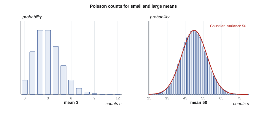
Two cautions apply. First, \(\sqrt{N}\) is the uncertainty of the raw count, not of a rate or a corrected result; it must be carried through every later step. Second, the square-root rule holds only for counts. It does not apply to a count rate, a dose rate, a meter reading or a number that has already been scaled. Taking the square root of 125 counts per minute is meaningless unless you know how many counts were actually recorded.

Propagating uncertainty

Results are almost always calculated from counts: rates, net rates after background, activities after efficiency correction. If a result \(u\) depends on independent measured quantities \(x, y, \ldots\), the standard propagation formula is

Four special cases cover most of counting-room work. For a sum or difference, the variances add: \(\sigma_{x \pm y}^2 = \sigma_x^2 + \sigma_y^2\). For multiplication or division by an exact constant, the standard deviation scales by the same constant. For a product or quotient of measured quantities, the relative variances add. And for a count rate \(r = N/t\) with an exactly known time, \(\sigma_r = \sqrt{N}/t = \sqrt{r/t}\).

The most important consequence is the net count rate. A sample counted for time \(t_g\) gives \(N_g\) gross counts; a background measured for \(t_b\) gives \(N_b\). The net rate and its uncertainty are

Subtracting background never reduces the uncertainty. It adds the background's own variance to the gross variance. When the net signal is small compared with background, the relative uncertainty of the net rate can be very large even when both counts are big.

# Counting statistics: Poisson uncertainty, net count rate, counting time split and Currie limits.
import math

# A smear sample counted for 10 min; background counted for 30 min.
gross, t_g = 1250, 10.0          # counts, minutes
bkg, t_b = 2700, 30.0
rg, rb = gross / t_g, bkg / t_b
net = rg - rb
sig = math.sqrt(gross / t_g**2 + bkg / t_b**2)
print(f"gross rate {rg:.1f} cpm, background {rb:.1f} cpm")
print(f"net rate {net:.1f} +/- {sig:.1f} cpm (1 sigma), relative {100*sig/net:.1f} %")

# Best split of a fixed 60 min between sample and background: t_s/t_b = sqrt(r_s/r_b)
T = 60.0
ratio = math.sqrt(rg / rb)
ts = T * ratio / (1 + ratio)
print(f"optimum split of {T:.0f} min: sample {ts:.1f} min, background {T-ts:.1f} min")

# Currie critical level and detection limit for paired counting (equal times), counts
for B in (10, 100, 1000):
    LC = 2.33 * math.sqrt(B)
    LD = 2.71 + 4.65 * math.sqrt(B)
    print(f"background {B:5d} counts: L_C = {LC:6.1f}, L_D = {LD:6.1f} counts")

gross rate 125.0 cpm, background 90.0 cpm
net rate 35.0 +/- 3.9 cpm (1 sigma), relative 11.2 %
optimum split of 60 min: sample 32.5 min, background 27.5 min
background    10 counts: L_C =    7.4, L_D =   17.4 counts
background   100 counts: L_C =   23.3, L_D =   49.2 counts
background  1000 counts: L_C =   73.7, L_D =  149.8 counts

Choosing counting times

Counting time is a resource. The counter is booked, samples queue, and an outage schedule waits for clearance results. If a fixed total time \(T\) must be shared between a sample and its background, the split that minimizes the uncertainty of the net rate is

For the smear above, \(\sqrt{125/90} = 1.18\), so a 60-minute allowance should be split as about 32.5 minutes on the sample and 27.5 minutes on background. The program shows the calculation. Two practical points follow. When the sample rate is much larger than background, almost all the time should go to the sample, and a background measured once per shift is adequate. When the sample is close to background, as in clearance and environmental work, the background deserves nearly as much time as the sample, and should be measured as close in time as possible because backgrounds drift.

The required time can also be found the other way: specify the relative precision you need on the net rate and solve for the time. Laboratories often set a target such as 10 % at the action level and adjust counting time automatically to reach it.

Decision limits and detection limits

Most of the smears in Marcel's stack are not obviously contaminated. Some give net counts of a few, some slightly negative. The question is no longer how precise the result is, but whether it shows any activity at all. Lloyd Currie's 1968 framework, now standard in health physics, answers that with two quantities that are often confused.

The critical level \(L_C\) is a decision threshold applied after counting. If the net count exceeds \(L_C\), the laboratory decides that activity is present. It is set so that a blank sample, with no activity, exceeds it only a small fraction of the time, conventionally 5 %. For paired counting with equal sample and background times and a background count \(B\), it is

The detection limit \(L_D\) is decided before counting. It is the smallest true net count that the procedure will detect with high probability, conventionally 95 %. With the same assumptions,

The constant 2.71 corrects for Poisson behaviour at low counts. Dividing \(L_D\) by efficiency, emission probability, counting time and sample size converts it to the minimum detectable activity (MDA), a property of the measurement method rather than of any one result.

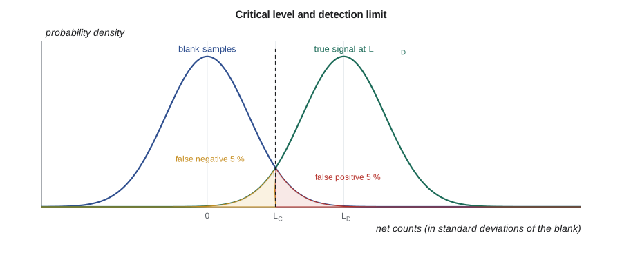
The two limits are used for different jobs. \(L_C\) decides whether a particular sample is reported as positive. \(L_D\) or the MDA tells a client, a regulator or a procedure writer what the method can detect, and must be below any clearance or action level that the measurement is meant to check. A frequent mistake is to report every result below the MDA as zero, or to compare a single result with the MDA instead of with \(L_C\). Another is to discard negative net results. A negative net count is a valid measurement of a sample near zero, and averaging must include it or the average will be biased high.

The program shows how the limits grow with background: for 100 background counts, \(L_C\) is 23 counts and \(L_D\) is 49. Halving background does not halve the MDA, because the limits scale with its square root. Shielding, low-background counters and longer counts all help, in proportion to the square root.

Testing a counting system

Poisson statistics also provide a check on the instrument itself. If a counter is working properly, repeated counts of a steady source should scatter by about \(\sqrt{N}\). Too much scatter points to electronic noise, a drifting high voltage or a loose cable. Too little scatter is just as suspicious and can indicate a counter that is saturating, a stuck register or results that have been copied. The chi-square test, introduced in lesson 11, makes the check quantitative and is part of a laboratory's routine quality control.

Under the CNSC's Radiation Protection Regulations, a licensee must be able to show how dose and contamination results were obtained. Marcel's procedures at Darlington therefore record raw counts and counting times, not only final results, so that every uncertainty can be reconstructed during an inspection.

Averaging repeated results

Monitoring programs often combine several results: four quarterly air filters, duplicate counts of the same sample, or readings from two detectors. When results have different uncertainties, a simple average gives too much weight to the poorest ones. The weighted mean uses weights equal to the inverse of each variance,

For counts of equal duration, the weighted mean reduces to the total counts divided by the total time, which is the simplest and safest way to combine them. Pooling the raw counts first and calculating once avoids rounding errors and handles small or zero counts properly.

A related judgment is whether two results agree. If two independent measurements differ by \(d\) and each has standard deviation \(\sigma_1\) and \(\sigma_2\), the difference has standard deviation \(\sqrt{\sigma_1^2 + \sigma_2^2}\). A difference more than about two of those standard deviations suggests a real change, such as contamination spreading between two surveys or a counter whose efficiency has shifted. Smaller differences are usually just counting scatter, and acting on them wastes effort. Marcel's rule of thumb for his staff is short: before you call something a trend, ask how large the difference is compared with its own uncertainty.

Rounding also deserves care. A result should be quoted with one or two significant figures in its uncertainty and the value rounded to match, such as \(35.0 \pm 3.9\) cpm rather than 35.0274 ± 3.94. Spurious digits suggest a precision the measurement does not have, while rounding too early in a chain of calculations introduces errors of its own, so intermediate values keep extra digits until the final report.

Dead time and other departures from Poisson

Real counters cannot record two events that arrive too close together. That dead time removes counts at high rates and changes the statistics slightly, because the recorded pulses are no longer independent. Lesson 7 treats it in detail. Other departures come from sources that are not stable during a count, such as short-lived radionuclides, which need decay correction, and from background that varies with radon progeny in the air or with nearby work. Good practice is to count backgrounds often and to know the expected range of every count.

Hana's sorting rule

By the end of the week Hana has a simple written method for the outage smears. Each smear is counted for a fixed time chosen so that the MDA is well below the station's contamination limit. The net count is compared with \(L_C\). Results above \(L_C\) are reported as activity with their uncertainty; results below are reported as less than the MDA, while the actual net value is kept in the database. Marcel approves it with one addition: any smear that is above \(L_C\) but within twice the uncertainty of the limit is recounted before an area is cleared or posted.