
NUC-310 · Lesson 11 of 12 · 19 min
Calibration and quality assurance
A measurement is only as good as the chain that connects it to a known standard. Marcel's counting room produces thousands of results a year that feed dose records, effluent reports, waste manifests and environmental reports, and any of them may be questioned years later. This lesson follows how the laboratory calibrates its instruments, how it estimates uncertainty, and how it shows, day after day, that its results can be trusted.
Traceability
A result is traceable when it can be related to a national or international measurement standard through an unbroken chain of calibrations, each with a stated uncertainty. For radioactivity, the top of the chain is a national metrology institute that realizes the becquerel by primary methods such as coincidence counting.
In Canada, the National Research Council's Metrology Research Centre maintains national standards for radioactivity and radiation dose, and calibration laboratories can be accredited against ISO/IEC 17025 through the Standards Council of Canada or the Canadian Association for Laboratory Accreditation.
Commercial suppliers prepare calibration sources whose activities are measured against those national standards and supplied with certificates stating activity, reference date and uncertainty. A laboratory's working standards, check sources and calibrated instruments then form the lower links of the chain. Every link must be documented: the source certificate, the date and conditions of calibration, and the instrument settings used.
Calibrating a gamma spectrometer
A germanium spectrometer needs three calibrations. The energy calibration relates channel to energy, the shape calibration relates peak width to energy, and the efficiency calibration relates counts in a full-energy peak to the number of photons emitted. Efficiency is the hardest, because it depends on photon energy and on the exact geometry: container size and shape, fill height, distance from the detector, and sample density and composition.
The usual method counts a mixed-radionuclide standard prepared in exactly the same container and matrix as the samples, with lines spread from below 100 keV to above 1.8 MeV. The measured efficiency at each energy is
where \(A\) is the certified activity decay-corrected to the counting date. The points are then fitted with a smooth function. Above about 200 keV, a straight line in log-log coordinates, \(\ln\varepsilon = a + b\ln E\), is often adequate; at lower energies, absorption in the detector's dead layer and the sample causes the curve to turn over, and polynomials in \(\ln E\) are used.
# Calibration and QA: efficiency fit vs energy, uncertainty budget and a chi-square check.
import math
pts = [(122, 0.0612), (344, 0.0331), (662, 0.0215), (1173, 0.0138), (1332, 0.0124)]
# fit ln(eff) = a + b ln(E) by least squares
xs = [math.log(e) for e, _ in pts]; ys = [math.log(f) for _, f in pts]
n = len(pts); mx = sum(xs) / n; my = sum(ys) / n
b = sum((x - mx) * (y - my) for x, y in zip(xs, ys)) / sum((x - mx)**2 for x in xs)
a = my - b * mx
for e, f in pts:
    fit = math.exp(a + b * math.log(e))
    print(f"{e:5d} keV: measured {f:.4f}, fit {fit:.4f}, diff {100*(f-fit)/fit:+5.1f} %")
print(f"efficiency(E) = {math.exp(a):.3f} * E^({b:.3f})")

# Combined standard uncertainty (relative, %)
budget = {'counting': 1.2, 'source activity': 1.5, 'efficiency fit': 2.0, 'geometry': 1.0, 'decay data': 0.3}
u = math.sqrt(sum(v**2 for v in budget.values()))
print(f"combined {u:.1f} %, expanded (k=2) {2*u:.1f} %")

# Chi-square test of 10 repeat counts
c = [1012, 987, 1030, 995, 1008, 971, 1019, 1001, 990, 1025]
m = sum(c) / len(c)
chi2 = sum((x - m)**2 for x in c) / m
print(f"mean {m:.1f}, chi-square {chi2:.2f} with 9 dof (accept 3.33 to 16.92 at 90 %)")122 keV: measured 0.0612, fit 0.0635, diff -3.6 % 344 keV: measured 0.0331, fit 0.0318, diff +4.2 % 662 keV: measured 0.0215, fit 0.0205, diff +4.8 % 1173 keV: measured 0.0138, fit 0.0140, diff -1.5 % 1332 keV: measured 0.0124, fit 0.0129, diff -3.6 % efficiency(E) = 1.568 * E^(-0.668) combined 3.0 %, expanded (k=2) 5.9 % mean 1003.8, chi-square 3.07 with 9 dof (accept 3.33 to 16.92 at 90 %)
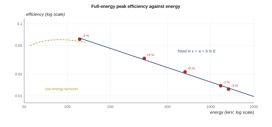
The program fits five calibration points and finds residuals of up to about 5 %, which is a little large for a careful calibration. Such residuals can come from coincidence summing (lesson 4) in nuclides with cascade emissions, from uncertain emission probabilities, or from an inadequate fit function. Marcel's laboratory accepts residuals of a few percent but investigates larger ones and applies summing corrections for nuclides such as cobalt-60 and europium-152 counted close to the detector.
When a matching standard cannot be made, for example for an unusual waste item, efficiency can be calculated with Monte Carlo modelling of the detector and sample, using a detector model validated against measured standards. The calculated efficiency then carries an additional uncertainty that reflects the model's validation.
Calibrating other instruments
Each instrument type has its own calibration. Survey meters are exposed to a calibrated gamma field, often from a caesium-137 source at known distances in a calibration range, and adjusted to read correctly within a tolerance on each scale. Their energy response is checked with lower-energy sources or X-ray beams. Contamination monitors are calibrated with large-area reference sources of known surface emission rate, and their efficiency is expressed per emitted particle and per unit area. Proportional counters are calibrated with alpha and beta standards on planchets of the same size as samples. Liquid scintillation counters use quenched standard sets to build quench curves. Dosimeters are irradiated to known doses in reference fields on phantoms, as part of the dosimetry service's performance testing.
Calibration intervals are set by procedure and by regulation, and instruments are also recalibrated after repair. Between calibrations, operational checks with a check source confirm that each instrument responds within a set range before use. A survey meter that fails its source check is tagged out of service.
Uncertainty budgets
A result reported without its uncertainty is incomplete. The international Guide to the Expression of Uncertainty in Measurement (GUM) provides the framework laboratories use. Each source of uncertainty is estimated as a standard uncertainty, either from statistics of repeated measurements (Type A) or from other information such as certificates, specifications or judgment (Type B). For a result that is a product or quotient of independent terms, the relative standard uncertainties combine in quadrature:
The combined standard uncertainty is multiplied by a coverage factor \(k\), usually 2, to give an expanded uncertainty corresponding to roughly 95 % confidence. In the program's budget, counting statistics contribute 1.2 %, the source activity 1.5 %, the efficiency fit 2.0 %, geometry 1.0 % and decay data 0.3 %, giving a combined uncertainty of 3.0 % and an expanded uncertainty of about 6 %. The budget shows where improvement would help: counting longer would barely change the total, while a better efficiency fit and a better standard would.
| Source of uncertainty | Type | How estimated |
|---|---|---|
| Counting statistics | A | Poisson √N on gross and background counts |
| Calibration source activity | B | Certificate value and coverage factor |
| Efficiency curve fit | A or B | Residuals of the fit or propagation of parameters |
| Sample geometry and density | B | Comparison of standards or modelling |
| Nuclear data (half-life, emission probability) | B | Evaluated data libraries |
| Timing and decay correction | B | Uncertainty in collection and counting times |
Quality control charts
Calibrations show that an instrument was right on one day. Quality control shows that it stays right. Every working day, each counter measures a check source in a fixed geometry, and each germanium detector records the position, width and area of check-source peaks. Results are plotted on control charts with a central line equal to the long-term mean and warning and action limits typically at two and three standard deviations. A result outside the action limits, or a trend such as seven successive results on one side of the mean, means the instrument is not used until the cause is found.
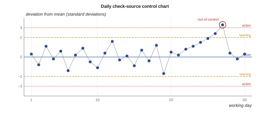
Background is charted the same way, because a rising background can mean contamination of the shield or detector. Germanium peak width charts catch electronic problems and loss of vacuum in the cryostat. Liquid scintillation counters chart the count rate of sealed standards and the quench indicator. Every chart has an owner who reviews it weekly.
The chi-square test
A counter can pass its check-source limits and still be misbehaving if its counts are more or less variable than Poisson statistics allow. The chi-square test compares the observed scatter of \(n\) repeat counts \(x_i\) with their mean \(\bar{x}\):
For a well-behaved counter, \(\chi^2\) follows the chi-square distribution with \(n - 1\) degrees of freedom. For ten counts, values between about 3.3 and 16.9 are expected 90 % of the time. The program's ten counts give 3.07, just below the lower limit. Too little scatter is unusual, and Marcel asks Hana to repeat the test. The second set falls inside the range, and the first is logged as a statistical outlier, which happens one time in twenty by definition. A second failure would have led to an investigation of the counter's electronics or of how the counts were recorded.
Laboratory quality systems
Calibration and quality control sit within a wider quality system. Laboratories accredited to ISO/IEC 17025 must document their methods, validate them, train and authorize staff, control their records, handle complaints and corrective actions, and be audited. Even unaccredited station laboratories follow the same principles because their results support regulatory submissions. Key elements include written procedures for every method, training records for every analyst, review of every result by a second person before release, and periodic internal audits.
External checks are equally important. Interlaboratory comparisons and proficiency tests send the same sample to many laboratories and compare the results with a reference value. Performance is usually scored by the difference from the reference divided by the combined uncertainty. Persistent bias in a laboratory's results, even within tolerance, is a signal to review its calibrations. Blind samples, prepared by the quality group and submitted as routine samples, test the whole process from sample receipt to report.
The CNSC expects licensees to have measurement quality assurance in their radiation protection and environmental programs, and dosimetry services must meet the management system requirements of REGDOC-2.7.2 Volume II.
Method validation
Before a laboratory uses a new method, or an old method on a new kind of sample, it validates it. Validation shows, with documented experiments, that the method measures what it claims to with the stated accuracy, precision and detection limit across the range of sample types it will meet. Typical tests include analysing reference materials of known activity, spiking real samples with known amounts and measuring recovery, repeating analyses on different days and by different analysts, and checking for interferences from other radionuclides or chemical components. The validation report sets the method's limits of applicability. A sample outside those limits, such as an unusually dense waste item, needs additional checks or a different method.
Validation is not done once and forgotten. Changes in detectors, software, chemical reagents or sample containers can affect a method, and a laboratory's change control process decides whether each change needs partial revalidation. Hana sees this when the counting room switches to a new brand of sample bottle: a short comparison with the old bottles, using the same standards, confirms that the efficiency calibration is unchanged before the new bottles enter routine use.
Software is part of the measurement system too. Spectrum analysis programs, liquid scintillation quench routines and dose calculation spreadsheets are verified with test cases whose answers are known, and each software version in use is recorded with the results it produced. When software is upgraded, a set of archived spectra is reanalysed and the results compared with the previous version before the new version is released for routine work.
Hana's audit
At the end of the lesson, Marcel gives Hana an internal audit to perform: pick three results from the past year, one effluent, one environmental and one waste, and trace each back to a national standard. She finds the counting records, the detector's control charts for the week, the efficiency calibration used, the source certificate and its reference to the national standard, and the analyst's training record. One calibration file is missing its review signature. Marcel calls it a minor finding, and the corrective action is closed within the week. The lesson he wants her to take away is that traceability is a paper trail as much as a physics problem.
Summary and key terms
- Traceability links each result to national standards through documented calibrations with stated uncertainties.
- Gamma spectrometers need energy, shape and geometry-specific efficiency calibrations.
- Efficiency ε = N_net/(A y t) is fitted vs energy, often as a straight line in log-log coordinates above 200 keV.
- Uncertainty budgets combine standard uncertainties in quadrature; expanded uncertainty usually uses k = 2.
- Control charts and chi-square tests show that instruments stay in control between calibrations.
- Accreditation, proficiency testing, blind samples and audits complete a quality system.
- Traceability
- The link between a result and a reference standard through an unbroken chain of calibrations.
- Efficiency calibration
- The relation between counts in a peak and photons emitted, for a given geometry.
- Standard uncertainty
- An uncertainty expressed as a standard deviation.
- Expanded uncertainty
- The combined standard uncertainty multiplied by a coverage factor.
- Control chart
- A plot of a check measurement over time with warning and action limits.
- Chi-square test
- A test comparing observed scatter with the scatter expected from Poisson statistics.
- Proficiency test
- An external test in which a laboratory analyses a sample of known value.
Practice problems
Work each problem on paper first, then reveal the answer to check.
A standard of 2000 Bq gives 4300 net counts in 1000 s at a line with y = 0.85. Efficiency?
Show answer
4300/(2000 × 0.85 × 1000) = 0.0025.
Combine 2 %, 2 % and 1 % relative uncertainties.
Show answer
√(4 + 4 + 1) = 3 %; expanded about 6 %.
Using the fitted curve in the program, estimate efficiency at 500 keV.
Show answer
1.568 × 500^−0.668 ≈ 0.0248.
Ten counts give χ² = 21. What does that suggest?
Show answer
More scatter than Poisson statistics allow; check for an instrument problem.
What is a Type B uncertainty?
Show answer
One estimated from information other than repeated measurements, such as a certificate.
Why are blind samples useful?
Show answer
They test the whole process from receipt to report without the analyst knowing.
Lesson quiz · 5 questions
Score 60% or more to complete this lesson.
Create a free account to save your progress, take quizzes and earn a certificate.