Meshing, convergence and stress singularities

In machine design, Owen found the stress concentration factor at the TP-80 shaft shoulder from a chart: with a fillet radius of 2.5 mm on a 35 mm shaft stepping up to 42 mm, r/d = 0.07 and D/d = 1.2 gave Kt of about 1.7 in bending. The heavier-duty shaft has a shoulder with a different ratio and a relief groove the charts do not cover, so its Kt must come from a finite element model. Before he trusts a number for the new shaft, Farah asks him to show that he can reproduce the old one, and to show how he knows the mesh is fine enough. This lesson is about that second question, the one that separates a credible stress analysis from a pretty picture.

The axisymmetric shoulder model

A shaft shoulder is a body of revolution, but bending is not axisymmetric: the stress varies around the circumference as the cosine of the angle. Most packages handle this with axisymmetric elements that accept nonsymmetric loads expanded in Fourier harmonics, or the analyst uses a three-dimensional model of a slice with symmetry. Owen uses the simplest equivalent that the charts themselves are based on: a model in which the nominal bending stress is applied at the remote ends, so that the ratio of peak to nominal stress is the stress concentration factor. The nominal bending stress in the 35 mm section, from the 216 N·m moment, is \(32M/\pi d^3 = 51.3\) MPa.

Meshing a fillet requires judgement. The stress peak sits on the fillet surface and decays within a fraction of the fillet radius, so elements there must be much smaller than the radius, while elements far away can be large. Owen uses quadratic elements with a local size set at the fillet surface and graded smoothly outward, so neighbouring elements differ in size by no more than a factor of about 1.5. Abrupt size changes create errors of their own. He runs three meshes with local element sizes of 1.0, 0.5 and 0.25 mm, halving the size each time, and reads the largest axial stress on the fillet.

Is it converged? Richardson extrapolation

Lesson 5 showed that for elements in their asymptotic range, the error is proportional to \(h^p\), where p is the order of convergence. With three meshes and a constant refinement ratio r, the order can be estimated from the results themselves, and the error removed by extrapolation. This procedure, named for Lewis Fry Richardson, who introduced it for finite difference calculations in 1910, is the standard way of quantifying discretization error:

where \(f_1, f_2, f_3\) are the coarse, medium and fine results. Patrick Roache proposed reporting the uncertainty in the fine-mesh result as a grid convergence index, \(\text{GCI} = F_s\,|(f_3 - f_2)/f_3|/(r^p - 1)\), with a safety factor \(F_s\) of 1.25 when three meshes are used. The GCI is now widely used in engineering computation and is recommended in verification guides for solid and fluid mechanics.

# Mesh convergence at the TP-80 shaft shoulder: Richardson extrapolation, the GCI, and a singular sharp corner
import math
M, d = 216.0, 0.035                                  # bending moment at the shoulder (N m) and smaller diameter (m)
s_nom = 32 * M / (math.pi * d**3) / 1e6               # nominal bending stress, MPa
print(f"Nominal bending stress at the shoulder: {s_nom:.2f} MPa")
# Peak axial stress at the 2.5 mm fillet from an axisymmetric model, local element size halved each time
h = [1.0, 0.5, 0.25]; s = [82.9, 86.1, 86.9]           # mm and MPa (Owen's three runs)
r = h[0] / h[1]
p = math.log((s[1] - s[0]) / (s[2] - s[1])) / math.log(r)
s_ext = s[2] + (s[2] - s[1]) / (r**p - 1)
gci = 1.25 * abs((s[2] - s[1]) / s[2]) / (r**p - 1)
print(f"Observed order of convergence p = {p:.2f} (theory about 2 for quadratic elements measured in stress)")
print(f"Richardson extrapolated peak stress {s_ext:.2f} MPa, so Kt = {s_ext/s_nom:.2f} (chart value 1.7)")
print(f"Grid convergence index on the finest mesh {100*gci:.2f} percent")
print("Fine-mesh error estimates: " + ", ".join(f"h = {hh} mm: {100*(s_ext-ss)/s_ext:.2f} %" for hh, ss in zip(h, s)))
# The same shoulder modelled with a sharp corner (no fillet): the stress never settles
hs = [1.0, 0.5, 0.25, 0.125]; ss = [98.0, 121.0, 150.0, 186.0]
print("\nSharp corner:  h (mm)   peak (MPa)   growth per halving")
for i, (a, b) in enumerate(zip(hs, ss)):
    g = f"{b/ss[i-1]:.3f}" if i else "  -  "
    print(f"               {a:6.3f}     {b:6.1f}        {g}")
lam = math.log(ss[-1] / ss[-2]) / math.log(2)
print(f"Stress grows roughly as h^-{lam:.2f}: a singularity, not a converging peak")
print(f"Linear elastic theory for a 90 degree re-entrant corner gives a stress exponent of about {1-0.5445:.2f}")
# Simple element quality checks for a quadrilateral: aspect ratio and the largest corner angle
def quality(pts):
    sides = [math.dist(pts[i], pts[(i+1) % 4]) for i in range(4)]
    angs = []
    for i in range(4):
        a, b, c = pts[i-1], pts[i], pts[(i+1) % 4]
        v1 = (a[0]-b[0], a[1]-b[1]); v2 = (c[0]-b[0], c[1]-b[1])
        angs.append(math.degrees(math.acos((v1[0]*v2[0] + v1[1]*v2[1]) / (math.hypot(*v1) * math.hypot(*v2)))))
    return max(sides) / min(sides), max(angs)
for name, q in (("good", [(0, 0), (1, 0), (1, 1), (0, 1)]), ("stretched", [(0, 0), (6, 0), (6, 1), (0, 1)]),
                ("skewed", [(0, 0), (1, 0), (2.2, 1), (1.2, 1)])):
    ar, amax = quality(q)
    print(f"{name:10s}: aspect ratio {ar:4.1f}, largest corner angle {amax:5.1f} degrees")

Nominal bending stress at the shoulder: 51.32 MPa
Observed order of convergence p = 2.00 (theory about 2 for quadratic elements measured in stress)
Richardson extrapolated peak stress 87.17 MPa, so Kt = 1.70 (chart value 1.7)
Grid convergence index on the finest mesh 0.38 percent
Fine-mesh error estimates: h = 1.0 mm: 4.89 %, h = 0.5 mm: 1.22 %, h = 0.25 mm: 0.31 %

Sharp corner:  h (mm)   peak (MPa)   growth per halving
                1.000       98.0          -  
                0.500      121.0        1.235
                0.250      150.0        1.240
                0.125      186.0        1.240
Stress grows roughly as h^-0.31: a singularity, not a converging peak
Linear elastic theory for a 90 degree re-entrant corner gives a stress exponent of about 0.46
good      : aspect ratio  1.0, largest corner angle  90.0 degrees
stretched : aspect ratio  6.0, largest corner angle  90.0 degrees
skewed    : aspect ratio  1.6, largest corner angle 140.2 degrees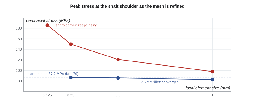

Owen's three results are 82.9, 86.1 and 86.9 MPa. The changes, 3.2 and then 0.8 MPa, fall by a factor of four as h halves, giving an observed order of 2.00, exactly what quadratic elements should show for stress. The extrapolated peak is 87.17 MPa, so Kt = 87.17/51.32 = 1.70, the chart value. The GCI of the finest mesh is 0.38 percent, and the estimated errors of the three meshes are 4.9, 1.2 and 0.3 percent. Owen now knows not only the answer but how good each mesh is: for the heavier-duty shaft, a 0.5 mm local size will give the peak to about one percent, which is adequate for a fatigue calculation whose other inputs are far less certain.

The important point is the order. If the observed order had come out as 0.4 or 5, or if the changes had not shrunk steadily, the meshes would not be in the asymptotic range and the extrapolation would mean nothing. In that case the cure is more refinement, smoother grading or a check for a modelling error, not a report of the finest result.

Stress singularities

Owen then repeats the study with the fillet removed, a perfectly sharp internal corner. The peak stress is 98 MPa with the coarsest mesh and grows by about 24 percent every time the mesh is halved, to 186 MPa at 0.125 mm, with no sign of levelling off. This is a stress singularity. Linear elasticity predicts that at a sharp re-entrant corner the stress is infinite, varying as \(r^{\lambda - 1}\) with distance r from the corner, where λ depends on the corner angle; for a 90 degree corner, the classical analysis by Max Williams gives λ ≈ 0.544, so the stress grows as \(r^{-0.46}\). A finite element mesh reports a finite stress at the corner only because each element averages over its own size, and the reported value grows without limit as the elements shrink.

Singularities appear in many places in practical models: sharp internal corners, the edge of a point load or point support, the tip of a crack, and the edge of a perfectly rigid support or a bonded joint between dissimilar materials. None of them represents real stress. Real corners have some radius, real loads are spread over an area, and real materials yield locally. The correct responses depend on why the stress is wanted. If the corner is a real design feature, model its actual radius, and if the radius is unknown, specify one on the drawing. If the singularity comes from an idealized support or load, read stresses away from it, at a distance of a few element sizes, where Saint-Venant's principle says the details no longer matter. If the corner is a crack, use fracture mechanics, which describes the singular field by a stress intensity factor instead of a stress.

The trap is a model that is not refined. A single mesh of a sharp corner gives a plausible-looking finite stress, and an analyst who does not refine it will never know that the number depends entirely on the element size. A convergence study exposes the problem at once, which is the strongest argument for always doing one at the locations that matter.

Element quality

The program's last part computes two quality measures for three quadrilaterals. The good element has an aspect ratio of 1 and right angles. The stretched element, six times longer than it is wide, has an aspect ratio of 6: acceptable along a shaft where the stress hardly changes axially, poor at the fillet. The skewed element has a reasonable aspect ratio, 1.6, but a corner angle of 140 degrees, close to the limit beyond which accuracy deteriorates. Meshers report statistics of these measures, and most let the user set limits that trigger local remeshing. Owen's rule from Farah is to check the quality of the elements at every location where a result will be reported, not just the average over the model.

Adaptive meshing and error estimates

Many packages estimate the discretization error of each element automatically, most commonly by comparing the raw element stresses with the smoothed nodal stresses, an approach associated with Olgierd Zienkiewicz and Jian Zhu. Some then refine the mesh automatically where the error is largest, repeating until a target is met. These tools are valuable, especially for large models, but they share the limitations of any convergence check: at a singularity, the error estimate stays high however much the mesh is refined, and an adaptive scheme will keep refining a corner whose stress is not real. The analyst still has to understand the geometry well enough to know which peaks are physical.