Heat transfer by finite elements

The mining customer runs some of its pumps on hot process water at up to 120 °C. In the standard TP-80, heat flows from the casing through a cast adapter into the bearing frame, and the bearing temperature is kept below its limit by the frame's surface losses. For the heavier-duty version, Farah wants to know how hot the adapter's far end gets, how much heat reaches the bearing frame, and whether the temperature difference across the casing produces thermal stress worth worrying about. All three questions are answered by finite element heat transfer analysis, which uses exactly the machinery of the previous lessons with temperature as the unknown. This lesson develops it, tests it against two exact solutions and shows how thermal results feed a stress model.

The conduction equation and its weak form

Steady heat conduction in a solid obeys Fourier's law, \(q = -k\nabla T\), and conservation of energy, which together give \(\nabla\cdot(k\nabla T) + Q = 0\), where Q is any internal heat generation. Boundaries can have a prescribed temperature, a prescribed heat flux or a convection condition \(q = h(T - T_\infty)\) to a surrounding fluid. Galerkin's method from Lesson 5 gives a weak form in which only first derivatives of T appear, and the shape functions of Lessons 2, 6 and 7 apply unchanged. The element matrix, now called the conductance matrix, is

where B now holds the temperature gradients of the shape functions and k is the thermal conductivity. The second term, from convection, makes the matrix depend on the film coefficient h as well as the conductivity, and the load vector gains a matching term \(\int hT_\infty N^{\mathsf{T}}\,dS\). Each node has one degree of freedom, its temperature, so thermal models are a third the size of structural models with the same mesh.

The adapter as a fin

The adapter is a cast ring joining the casing to the bearing frame, and heat flows along it while leaking from its outer surface to the surrounding air. One-dimensionally, it behaves like a fin, a problem with a well-known exact solution. Owen represents it by an equivalent steel bar 0.12 m long with conductivity 45 W/m·K, cross-sectional area 1.2 × 10⁻³ m² and a wetted perimeter of 0.40 m, with the base held at the 120 °C casing temperature and air at 25 °C on the sides and the end, with a film coefficient of 12 W/m²·K, a typical value for still air with some radiation. The fin parameter is \(m = \sqrt{hP/kA} = 9.43\) m⁻¹, so mL = 1.13, and the exact solution, including convection from the end face, gives an end temperature of 79.27 °C and a heat flow into the adapter of 39.71 W.

The finite element model uses two-node elements along the bar. Each has the conduction matrix of a bar, \((kA/l)\begin{bmatrix} 1 & -1 \\ -1 & 1\end{bmatrix}\), plus the side-convection matrix \((hPl/6)\begin{bmatrix} 2 & 1 \\ 1 & 2\end{bmatrix}\). The end face adds hA to the last diagonal term. The base temperature is prescribed, like a support, and the heat flow into the adapter is recovered from the base node's row, exactly as a reaction force was recovered in Lesson 1.

# Heat transfer by finite elements: the casing-to-bearing-frame adapter as a fin, and 2D conduction in a square
import math
def solve(A, b):
    n = len(b); A = [r[:] for r in A]; b = b[:]
    for k in range(n):
        p = max(range(k, n), key=lambda i: abs(A[i][k])); A[k], A[p] = A[p], A[k]; b[k], b[p] = b[p], b[k]
        for i in range(k + 1, n):
            f = A[i][k] / A[k][k]
            if f:
                for j in range(k, n): A[i][j] -= f * A[k][j]
                b[i] -= f * b[k]
    x = [0.0] * n
    for i in range(n - 1, -1, -1): x[i] = (b[i] - sum(A[i][j] * x[j] for j in range(i + 1, n))) / A[i][i]
    return x
# Adapter: equivalent steel bar k 45 W/m K, area 1.2e-3 m^2, wetted perimeter 0.40 m, length 0.12 m,
# base at the 120 C casing, air at 25 C with h = 12 W/m^2 K on the sides and the end
k, Ac, Pm, L, h, Tb, Ta = 45.0, 1.2e-3, 0.40, 0.12, 12.0, 120.0, 25.0
m = math.sqrt(h * Pm / (k * Ac))
def exact(x):
    return Ta + (Tb - Ta) * (math.cosh(m*(L-x)) + h/(m*k) * math.sinh(m*(L-x))) / (math.cosh(m*L) + h/(m*k) * math.sinh(m*L))
q_exact = k * Ac * m * (Tb - Ta) * (math.sinh(m*L) + h/(m*k) * math.cosh(m*L)) / (math.cosh(m*L) + h/(m*k) * math.sinh(m*L))
def fin(ne):
    n = ne + 1; le = L / ne; K = [[0.0] * n for _ in range(n)]; F = [0.0] * n
    for e in range(ne):
        kc, kh = k * Ac / le, h * Pm * le / 6      # conduction and side-convection element matrices
        for a, b, v in ((e, e, kc + 2*kh), (e+1, e+1, kc + 2*kh), (e, e+1, -kc + kh), (e+1, e, -kc + kh)): K[a][b] += v
        F[e] += h * Pm * le / 2 * Ta; F[e+1] += h * Pm * le / 2 * Ta
    K[-1][-1] += h * Ac; F[-1] += h * Ac * Ta       # convection from the end face
    rhs = [F[i] - K[i][0] * Tb for i in range(1, n)]
    T = [Tb] + solve([r[1:] for r in K[1:]], rhs)
    q = sum(K[0][j] * T[j] for j in range(n)) - F[0]   # heat entering at the base = reaction at the fixed node
    return T, q
print(f"m = {m:.2f} 1/m, mL = {m*L:.3f}; exact end temperature {exact(L):.2f} C, heat flow {q_exact:.2f} W")
for ne in (1, 2, 4, 8):
    T, q = fin(ne)
    print(f"  {ne} elements: end temperature {T[-1]:7.2f} C, heat into the adapter {q:6.2f} W ({100*(q-q_exact)/q_exact:+.2f} %)")

# 2D steady conduction in a square plate: one edge held at 100 C, the other three at 0 C.
# By symmetry and superposition the exact centre temperature is 25 C. Linear triangles on an n x n grid.
def square(n):
    hgrid = 1.0 / n; nid = lambda i, j: j * (n + 1) + i; N = (n + 1)**2
    K = [[0.0] * N for _ in range(N)]
    for j in range(n):
        for i in range(n):
            for tri in ((nid(i, j), nid(i+1, j), nid(i+1, j+1)), (nid(i, j), nid(i+1, j+1), nid(i, j+1))):
                xy = [((t % (n+1)) * hgrid, (t // (n+1)) * hgrid) for t in tri]
                (x1, y1), (x2, y2), (x3, y3) = xy
                A2 = (x2-x1)*(y3-y1) - (x3-x1)*(y2-y1); b = [y2-y3, y3-y1, y1-y2]; c = [x3-x2, x1-x3, x2-x1]
                for p in range(3):
                    for q in range(3): K[tri[p]][tri[q]] += (b[p]*b[q] + c[p]*c[q]) / (2 * A2)
    Tfix = {}
    for i in range(n + 1):
        Tfix[nid(i, 0)] = 0.0; Tfix[nid(0, i)] = 0.0; Tfix[nid(n, i)] = 0.0
    for i in range(1, n): Tfix[nid(i, n)] = 100.0
    free = [a for a in range(N) if a not in Tfix]
    rhs = [-sum(K[a][b] * v for b, v in Tfix.items()) for a in free]
    T = dict(Tfix); T.update(zip(free, solve([[K[a][b] for b in free] for a in free], rhs)))
    return T[nid(n // 2, n // 2)], T[nid(n // 2, 3 * n // 4)]
ex = sum(400 / (j * math.pi) * math.sinh(j * math.pi * 0.75) / math.sinh(j * math.pi) * math.sin(j * math.pi * 0.5) for j in range(1, 80, 2))
print(f"Exact series at (0.5, 0.75): {ex:.3f} C")
for n in (4, 8, 16):
    c, q = square(n)
    print(f"Square, {n:2d} x {n:<2d} grid ({2*n*n:3d} triangles): centre {c:6.3f} C, point (0.5, 0.75) {q:6.3f} C, error {q-ex:+.3f} C")

m = 9.43 1/m, mL = 1.131; exact end temperature 79.27 C, heat flow 39.71 W
  1 elements: end temperature   76.23 C, heat into the adapter  42.85 W (+7.93 %)
  2 elements: end temperature   78.59 C, heat into the adapter  40.47 W (+1.93 %)
  4 elements: end temperature   79.10 C, heat into the adapter  39.90 W (+0.48 %)
  8 elements: end temperature   79.23 C, heat into the adapter  39.75 W (+0.12 %)
Exact series at (0.5, 0.75): 54.053 C
Square,  4 x 4  grid ( 32 triangles): centre 25.000 C, point (0.5, 0.75) 52.679 C, error -1.374 C
Square,  8 x 8  grid (128 triangles): centre 25.000 C, point (0.5, 0.75) 53.608 C, error -0.445 C
Square, 16 x 16 grid (512 triangles): centre 25.000 C, point (0.5, 0.75) 53.933 C, error -0.120 C

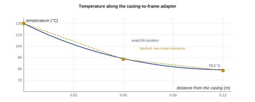
One element gives an end temperature 3 °C low and a heat flow 7.9 percent high; two elements reduce the heat flow error to 1.9 percent, and eight to 0.12 percent. The heat flow error falls by a factor of four each time the elements are halved, the h² behaviour of a quantity that, like strain energy, is an integral over the whole model. The bearing frame receives about 40 W through the adapter, a small fraction of the pump's losses, so Owen concludes that the adapter will not overheat the bearings. A full three-dimensional thermal model of the frame would refine this, but the one-dimensional model has already answered the design question to within a few percent.

Two-dimensional conduction

The program's second model is a classic test: a square plate with one edge held at 100 °C and the other three at 0 °C. By symmetry and superposition, adding the four rotated versions of the problem gives a plate with all edges at 100 °C, which is 100 °C everywhere, so the centre of the original plate must be exactly 25 °C. The exact temperature anywhere else is a Fourier series, and at the point halfway across and three quarters of the way toward the hot edge it is 54.05 °C.

The program meshes the square with linear triangles. The centre temperature comes out as exactly 25 °C on every mesh, because the triangle mesh used here reproduces the discrete symmetry of the problem, a useful sanity check but not a proof of accuracy. At the off-centre point the error falls from 1.37 °C on the 4 × 4 grid to 0.45 and 0.12 °C as the grid is halved, approaching the factor of four expected for linear elements. A test with a symmetry-guaranteed answer and one without is a good pair: the first catches assembly and boundary condition errors, the second measures accuracy.

Transient heat transfer

When the pump starts on hot water, the casing heats up over several minutes, and the stresses during that transient can exceed the steady-state ones, because the inside of the casing is hot while the outside is still cold. Transient analysis adds a capacitance matrix, \(C = \int \rho c\,N^{\mathsf{T}}N\,dV\), analogous to the mass matrix of Lesson 11, giving \(C\dot{T} + KT = F\). This is solved by stepping in time. The common family of methods, the θ-method, includes the explicit forward Euler scheme (θ = 0), the Crank-Nicolson scheme (θ = 1/2) and the implicit backward Euler scheme (θ = 1). Explicit schemes are simple but become unstable if the time step exceeds a limit proportional to the square of the smallest element size; implicit schemes are unconditionally stable but need a matrix solve each step, and Crank-Nicolson can produce oscillations near sudden changes. For a casing warm-up, backward Euler with time steps of a few seconds is a robust choice.

The time scale of a transient can be estimated by hand before modelling. The thermal diffusivity of steel is about \(1.2 \times 10^{-5}\) m²/s, so a 20 mm casing wall reaches near-uniform temperature in a time of the order of \(L^2/\alpha = 0.02^2/1.2 \times 10^{-5} \approx 33\) s after its inner surface is heated, and the whole casing, much of whose heating depends on surface convection, takes several minutes. A transient model whose results disagree with such an estimate by an order of magnitude needs to be checked.

From temperature to thermal stress

Thermal stress analysis uses the temperature field as a load. The usual workflow is sequential: run the thermal model, then map its nodal temperatures onto a structural model, often the same mesh, and apply them as initial strains \(\alpha(T - T_{ref})\), as Lesson 2 did for a single bar. Farah asks Owen to check the steady-state stress from the casing's through-wall temperature difference. A useful hand estimate for a plate whose faces differ by ΔT and whose edges cannot rotate is \(\sigma = E\alpha\Delta T/(2(1 - \nu))\). For the casing wall, with water at 120 °C inside and a film-limited outer surface, the thermal model shows a through-wall difference of about 4 °C, giving \(200\,000 \times 12 \times 10^{-6} \times 4/1.4 \approx 7\) MPa. That is small, so steady thermal stress is not a concern; the start-up transient, when the difference briefly reaches tens of degrees, is the case that needs checking against the casting's fatigue strength.

Getting thermal boundary conditions right

Thermal models are only as good as their film coefficients, which depend on fluid velocity, geometry and orientation and are rarely known better than to within 20 to 50 percent. Correlations from heat transfer texts, which Owen used in his heat transfer course, are the usual source. Because the uncertainty is large, a thermal analysis should report the sensitivity of its key results to h, for example by running the model at the expected value and at half and double. For the adapter, the heat flow changes by much less than the film coefficient does, because the conduction resistance of the adapter also limits it, which is reassuring. Radiation is often included as an increment to h near the surface temperature, or modelled exactly as a nonlinear boundary condition.