The finite element method and the direct stiffness approach

Owen Clarke has been at Tidewater Pump Works in Moncton for most of a year now as a junior engineer. He has instrumented the TL-3 test stand, written up the witnessed test of six TP-80 pumps and learned to trust measurements only as far as their uncertainty allows. His next assignment comes from Farah Siddiqui, the senior design engineer. The TP-80 is being offered in a heavier-duty version for a mining customer, with a fabricated baseplate, a new casing cover rated for a higher test pressure and a longer motor bracket. Some of that can be checked with the hand calculations Owen used in machine design and vibrations. Some of it cannot: the baseplate is a welded frame of channels and plates, the cover is a ribbed casting with bolt holes and a gasket groove, and the stress at the shaft shoulder depends on a fillet only a few millimetres across.

For shapes like these, engineers use the finite element method, usually through a commercial or open-source software package. Farah's condition for letting Owen run those packages is simple. Before he uses one on a TP-80 part, he must understand what it is doing well enough to build a small version himself, and every result he reports must be checked by a method that does not depend on the software. This course follows that apprenticeship. Each lesson builds one piece of the method in a few dozen lines of Python, checks it against an answer known from hand calculation, and then applies the idea to a part of the heavier-duty TP-80. By the end Owen, and the reader, will be able to plan an analysis, judge a mesh, recognize when a result is wrong and write the kind of verification record a professional engineer would sign.

What the finite element method does

The governing equations of solid mechanics and heat transfer are partial differential equations. For a bar, a beam or a plate with a simple shape they can be solved exactly, which is why handbooks are full of formulas for those cases. A real part has a shape no formula describes. The finite element method replaces the continuous part by a collection of small, simple pieces called elements, joined at points called nodes. Within each element the unknown field, such as displacement or temperature, is assumed to vary in a simple way, usually linearly or quadratically, and is described entirely by its values at the element's nodes. The infinite number of unknowns in the real part becomes a finite number of nodal values, called degrees of freedom, and the differential equations become a system of algebraic equations, one for each degree of freedom.

For linear static problems the system takes the form \(K u = F\), where u is the vector of unknown nodal displacements, F the vector of nodal forces and K the global stiffness matrix. Solving it gives the displacements, and from them every other quantity: strains from how the displacements vary across each element, stresses from the material law, reactions at the supports from the rows of the system that belong to restrained nodes. Heat conduction gives the same structure with temperatures in place of displacements, heat flows in place of forces and a conductance matrix in place of stiffness. Vibration adds a mass matrix and leads to an eigenvalue problem. The idea is the same in every case: approximate locally, assemble globally, solve.

The method grew out of aircraft structural analysis in the 1950s, when engineers needed to analyse swept wings that no beam formula described, and it was given a firm mathematical foundation in the following decades. The term finite element is generally credited to Ray Clough around 1960. Today the same ideas run inside every structural, thermal and multiphysics package used in industry, from the solvers built into computer-aided design programs to the specialized codes used for crash and fluid analysis. Learning the method rather than one package means a student can move between packages and, more importantly, can recognize when any of them is being misused.

The workflow

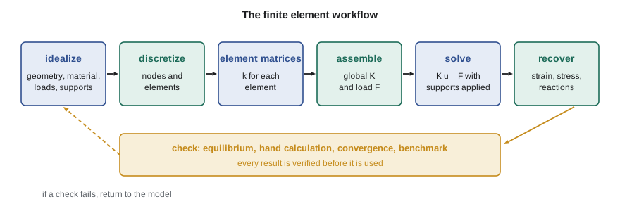
Every finite element analysis, whether of a spring or an engine block, passes through the same stages. Idealization comes first and is the most important: the engineer decides what physical problem to solve. Which parts are included, and which are replaced by supports or loads? Is the material linear elastic, and is the deformation small? Is the problem two-dimensional, axisymmetric or fully three-dimensional? Is a bolt modelled as a solid, a beam, a spring or not at all? These decisions are made before the software opens, and no amount of mesh refinement repairs a wrong one.

Discretization divides the idealized geometry into elements and nodes. Element matrices are then formed for each element from its geometry and material: a small stiffness matrix relating its nodal forces to its nodal displacements. Assembly adds every element matrix into the global matrix at the rows and columns of the element's degrees of freedom, and gathers the loads into the global force vector. Supports are applied by fixing the displacements of restrained degrees of freedom. The reduced system is solved, and the results are recovered and displayed. Finally, and in Farah's group always, the results are checked: does the sum of the reactions equal the applied load, does a hand calculation give the same order of answer, does the answer settle as the mesh is refined, does the software reproduce a published benchmark?

The spring element

The simplest element is a linear spring joining two nodes, each of which can move only along the spring's axis. Call the nodal displacements \(u_1\) and \(u_2\) and the forces applied at the nodes \(f_1\) and \(f_2\). The spring stretches by \(u_2 - u_1\), so it carries a tension \(k(u_2 - u_1)\). Node 2 is pulled back by that tension and node 1 is pulled forward, so equilibrium of each node gives

The 2 by 2 matrix is the element stiffness matrix. It has properties shared by every stiffness matrix in this course. It is symmetric, a consequence of the reciprocity of linear elastic systems (Maxwell's reciprocal theorem). Each row sums to zero, because moving both nodes by the same amount is a rigid-body motion that produces no force. And it is singular: on its own, the spring can drift freely, so the matrix cannot be inverted until at least one node is restrained. A finite element model that is not supported against every rigid-body motion gives a singular global matrix, and a solver will either stop with an error or return enormous, meaningless displacements. Checking for that condition is one of the first diagnostic habits an analyst learns.

Assembly by the direct stiffness method

A structure made of several springs is assembled node by node. Number the nodes, and for each spring add its four stiffness terms into the global matrix at the rows and columns of its two nodes. Where several springs meet at a node, their contributions add, because the force needed to hold a node in a displaced position is the sum of the forces from all the springs attached to it. This process, called the direct stiffness method, is exactly what commercial software does for millions of elements; only the bookkeeping is more elaborate.

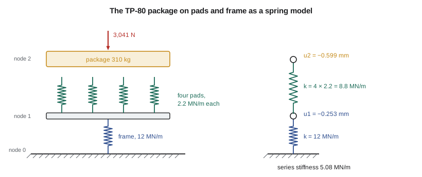
Owen's first model is one he already knows the answer to. In the vibrations course the TP-80 package, 310 kg of pump, motor and baseplate, sat on four rubber pads of 2.2 MN/m each, mounted on a steel frame whose own stiffness was about 12 MN/m. The three-node model has the floor as node 0, the top of the frame as node 1 and the baseplate as node 2. The frame is one spring from node 0 to node 1; the four pads are four springs from node 1 to node 2. Assembly gives a 3 by 3 matrix with 12 MN/m at the (0,0) position, 12 + 4 × 2.2 = 20.8 MN/m at (1,1), 8.8 MN/m at (2,2) and the negative cross terms between connected nodes. The weight, 310 × 9.81 = 3,041 N, acts downward at node 2.

Supports, solution and reactions

Node 0 is fixed to the floor, so its displacement is zero. The standard way to apply that condition is to partition the system: the rows and columns of free degrees of freedom form a smaller, nonsingular matrix \(K_{ff}\), which is solved for the free displacements. The rows belonging to the fixed degrees of freedom are then used afterwards to find the reactions, \(R = K u - F\) evaluated at those rows. Commercial codes use the same idea, sometimes implemented by replacing a fixed row with a large number on the diagonal (the penalty method), which is simpler to program but slightly approximate.

Solving the 2 by 2 free system by Gaussian elimination is the heart of the program below. Gaussian elimination reduces the matrix to upper triangular form by subtracting multiples of each row from those below it, then finds the unknowns by back substitution. The program swaps rows to put the largest available number on the diagonal, a precaution called partial pivoting that keeps rounding errors small. Real finite element solvers exploit the fact that a stiffness matrix is sparse, with most entries zero, and symmetric, and use specialized direct or iterative methods that handle millions of equations. The arithmetic idea is unchanged.

# Direct stiffness method for a chain of springs: assemble, apply supports, solve, recover forces
def solve(A, b):
    """Gaussian elimination with partial pivoting (A and b are copied)."""
    n = len(b); A = [row[:] for row in A]; b = b[:]
    for k in range(n):
        p = max(range(k, n), key=lambda i: abs(A[i][k])); A[k], A[p] = A[p], A[k]; b[k], b[p] = b[p], b[k]
        for i in range(k + 1, n):
            f = A[i][k] / A[k][k]
            for j in range(k, n): A[i][j] -= f * A[k][j]
            b[i] -= f * b[k]
    x = [0.0] * n
    for i in range(n - 1, -1, -1):
        x[i] = (b[i] - sum(A[i][j] * x[j] for j in range(i + 1, n))) / A[i][i]
    return x

def spring_model(nnodes, elements, fixed, loads):
    K = [[0.0] * nnodes for _ in range(nnodes)]
    for i, j, k in elements:                       # element stiffness k[[1,-1],[-1,1]] added at rows/columns i, j
        K[i][i] += k; K[j][j] += k; K[i][j] -= k; K[j][i] -= k
    free = [n for n in range(nnodes) if n not in fixed]
    Kff = [[K[a][b] for b in free] for a in free]
    uf = solve(Kff, [loads.get(n, 0.0) for n in free])
    u = [0.0] * nnodes
    for n, v in zip(free, uf): u[n] = v
    R = {n: sum(K[n][m] * u[m] for m in range(nnodes)) - loads.get(n, 0.0) for n in fixed}
    forces = [k * (u[j] - u[i]) for i, j, k in elements]
    return u, R, forces

# Model 1: TP-80 package on four rubber pads (2.2 MN/m each) sitting on a frame of stiffness 12 MN/m
W = 310 * 9.81                                    # package weight, N (acts downward, taken as negative)
elements = [(0, 1, 12e6)] + [(1, 2, 2.2e6)] * 4   # node 0 floor, node 1 frame top, node 2 baseplate
u, R, f = spring_model(3, elements, fixed=[0], loads={2: -W})
print(f"Package weight {W:.0f} N")
print(f"Frame top moves {1000*u[1]:.3f} mm, baseplate moves {1000*u[2]:.3f} mm")
print(f"Floor reaction {R[0]:.0f} N (equals the weight: equilibrium check)")
print(f"Force in each pad {f[1]:.0f} N, in the frame {f[0]:.0f} N")
k_eq = W / -u[2]
print(f"Equivalent stiffness {k_eq/1e6:.3f} MN/m; hand formula 1/(1/12 + 1/8.8) = {1/(1/12 + 1/8.8):.3f} MN/m")

# Model 2: three springs in a line (stiffness in N/mm), both ends held, 500 N at node 1 (a textbook check)
u, R, f = spring_model(4, [(0, 1, 1000.0), (1, 2, 2000.0), (2, 3, 3000.0)], fixed=[0, 3], loads={1: 500.0})
print(f"\nModel 2 displacements (mm): " + ', '.join(f"{x:.4f}" for x in u))
print(f"Reactions (N): left {R[0]:.2f}, right {R[3]:.2f}, sum {R[0] + R[3]:.2f} against applied 500")
print("Element forces (N, tension positive): " + ', '.join(f"{x:.2f}" for x in f))

Package weight 3041 N
Frame top moves -0.253 mm, baseplate moves -0.599 mm
Floor reaction 3041 N (equals the weight: equilibrium check)
Force in each pad -760 N, in the frame -3041 N
Equivalent stiffness 5.077 MN/m; hand formula 1/(1/12 + 1/8.8) = 5.077 MN/m

Model 2 displacements (mm): 0.0000, 0.2273, 0.0909, 0.0000
Reactions (N): left -227.27, right -272.73, sum -500.00 against applied 500
Element forces (N, tension positive): 227.27, -272.73, -272.73

The program confirms what Owen expected. The baseplate settles by 0.599 mm, of which 0.253 mm is the frame and the rest the pads. The floor reaction equals the weight, the first and most basic check of any static analysis. Each pad carries a quarter of the load, 760 N, and the equivalent stiffness of 5.077 MN/m matches the series formula \(1/(1/12 + 1/8.8)\) from the vibrations course. A finite element program has reproduced a hand calculation exactly, as it should: for springs, the element is not an approximation at all.

The second model is a textbook check with a load in the middle of a chain held at both ends. The reactions come out as 227.27 N and 272.73 N, both pointing against the load and adding up to it. The middle spring and the right-hand spring carry the same compressive force, which they must, since no load is applied at the node between them. Signs deserve care in every program: here a positive element force means tension, and the reactions are the forces the supports apply to the structure. Mixing sign conventions is one of the commonest sources of error when results are transferred from software to a report.

Why bother with a program for springs?

For three springs, writing a program is more work than solving by hand. The point is that the same assembly loop, unchanged, will handle three thousand springs, or three million elements of any type, because each element is treated alone and its contribution simply added. The hand method does not scale; the stiffness method does. A second point is less obvious: by building the method from the bottom, Owen learns where its errors come from. The spring element is exact, so every error in this lesson would be a modelling or programming error. In later lessons the elements themselves become approximate, and separating approximation error from mistakes becomes the central skill of the analyst.

The process also teaches what software hides. A package will accept a model with a missing support and return huge displacements, or a model with a unit error and return stresses a thousand times too large, without complaint. The analyst's defence is a set of independent checks: reactions that sum to the applied load, deflections of the right order from a hand estimate, a mesh that has been refined until the answer stops changing. The rest of this course adds to that set of checks lesson by lesson.

Responsibility for the result

In Canada, engineering work on equipment such as a pump sold for an industrial site is usually reviewed and sealed by a professional engineer (P.Eng.). The regulator here is Engineers and Geoscientists New Brunswick. The seal attests that the engineer is responsible for the work, including any calculation done by software. Engineering regulators have published guidance on this point; Professional Engineers Ontario's guideline on using software-based engineering tools, for example, makes clear that software is a tool and that the engineer remains responsible for understanding its assumptions, verifying its results and documenting the checks made. Owen is not yet licensed, so Farah will review and seal his work, but she expects his records to show exactly how each result was checked.