Isoparametric elements and numerical integration

The constant-strain triangle has straight sides and constant strain, and the integral that gives its stiffness can be done by hand. Better elements have strains that vary, sides that may be curved and integrals that cannot be evaluated in closed form for a general shape. The solution adopted by essentially every finite element program, developed in the 1960s, is the isoparametric element: every element is treated as a distorted copy of a simple parent shape, a square or a cube, and its integrals are evaluated numerically by Gauss quadrature at a few points inside the parent. This lesson builds the four-node quadrilateral, the Q4, in that way, explains what the Jacobian and the integration points are, and shows why element shape matters.

The parent element and the mapping

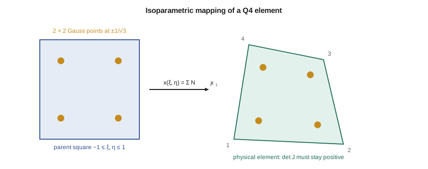
The parent element is a square in natural coordinates ξ and η, each running from −1 to 1. The bilinear shape functions

where \((\xi_i, \eta_i)\) are the parent corner coordinates, equal one at their own corner and zero at the others. The element is called isoparametric because the same functions serve two purposes: they interpolate the displacement from the nodal values, \(u = \sum N_i u_i\), and they map the parent square onto the real element, \(x = \sum N_i x_i\), \(y = \sum N_i y_i\). A square maps to any convex quadrilateral. With eight-node quadratic shape functions, a parent square maps to an element with curved sides, which fits a fillet or bore far better than straight-sided elements.

The Jacobian

Strains need derivatives with respect to x and y, but the shape functions are written in ξ and η. The chain rule connects them through the Jacobian matrix of the mapping:

Its determinant, det J, is the ratio of a small area in the real element to the corresponding area in the parent, so \(dx\,dy = \det J\,d\xi\,d\eta\). For a square element 10 mm on a side, det J is 25 everywhere: the real area of 100 mm² is 25 times the parent's area of 4. For a distorted element, det J varies from point to point. If any part of the element is folded back on itself, as happens when one corner is pushed inward past the line joining its neighbours, det J becomes negative there. The mapping is then not one-to-one, and the stiffness matrix is meaningless. Software checks det J at every integration point and refuses to solve, or reports a distorted element, when it is zero or negative.

Gauss quadrature

The element stiffness becomes an integral over the parent square, \(k = \int_{-1}^{1}\int_{-1}^{1} B^{\mathsf{T}}DB\,t\,\det J\,d\xi\,d\eta\), whose integrand is a ratio of polynomials for a distorted element. It is evaluated numerically. Carl Friedrich Gauss showed that with n carefully placed points and weights, the integral of any polynomial up to degree 2n − 1 over [−1, 1] is exact. One point at the centre, weight 2, integrates linear functions exactly; two points at \(\pm 1/\sqrt{3}\), weight 1, integrate cubics; three points at 0 and \(\pm\sqrt{0.6}\), weights 8/9 and 5/9, integrate fifth-degree polynomials. In two dimensions the rule is applied in each direction, so the Q4 uses a 2 × 2 grid of four points and quadratic elements usually a 3 × 3 grid.

# Isoparametric quadrilaterals and Gauss quadrature: exactness, the Jacobian, and Q4 elements in bending
import math
GP = {1: [(0.0, 2.0)], 2: [(-1/math.sqrt(3), 1.0), (1/math.sqrt(3), 1.0)],
      3: [(-math.sqrt(0.6), 5/9), (0.0, 8/9), (math.sqrt(0.6), 5/9)]}
print("Gauss quadrature of x^k on [-1, 1]:  k   exact     1 point   2 points   3 points")
for k in range(7):
    ex = 0.0 if k % 2 else 2 / (k + 1)
    vals = [sum(w * x**k for x, w in GP[n]) for n in (1, 2, 3)]
    print(f"                                   {k}   {ex:7.4f}   " + "   ".join(f"{v:7.4f}" for v in vals))
def shape(xi, eta):
    N = [(1-xi)*(1-eta)/4, (1+xi)*(1-eta)/4, (1+xi)*(1+eta)/4, (1-xi)*(1+eta)/4]
    dxi = [-(1-eta)/4, (1-eta)/4, (1+eta)/4, -(1+eta)/4]; deta = [-(1-xi)/4, -(1+xi)/4, (1+xi)/4, (1-xi)/4]
    return N, dxi, deta
def jac(xy, xi, eta):
    _, a, b = shape(xi, eta)
    J = [[sum(a[i]*xy[i][0] for i in range(4)), sum(a[i]*xy[i][1] for i in range(4))],
         [sum(b[i]*xy[i][0] for i in range(4)), sum(b[i]*xy[i][1] for i in range(4))]]
    return J, J[0][0]*J[1][1] - J[0][1]*J[1][0]
for name, xy in (("square 10 x 10 mm", [(0, 0), (10, 0), (10, 10), (0, 10)]),
                 ("distorted", [(0, 0), (10, 0), (7, 8), (0, 10)]),
                 ("re-entrant corner (bad)", [(0, 0), (10, 0), (3, 3), (0, 10)])):
    dets = [jac(xy, x, y)[1] for x, _ in GP[2] for y, _ in GP[2]]
    area = sum(jac(xy, x, y)[1] for x, _ in GP[2] for y, _ in GP[2])
    print(f"{name:25s}: det J at the 2x2 Gauss points " + ", ".join(f"{d:6.2f}" for d in dets) + f"; area by quadrature {area:.1f} mm^2")

# Q4 plane-stress cantilever, same plate as Lesson 6 (200 x 50 x 10 mm, 1 kN), full 2x2 integration
def solve(A, b):
    n = len(b); A = [r[:] for r in A]; b = b[:]
    for k in range(n):
        p = max(range(k, n), key=lambda i: abs(A[i][k])); A[k], A[p] = A[p], A[k]; b[k], b[p] = b[p], b[k]
        for i in range(k + 1, n):
            f = A[i][k] / A[k][k]
            if f:
                for j in range(k, n): A[i][j] -= f * A[k][j]
                b[i] -= f * b[k]
    x = [0.0] * n
    for i in range(n - 1, -1, -1): x[i] = (b[i] - sum(A[i][j] * x[j] for j in range(i + 1, n))) / A[i][i]
    return x
E, nu, t, Lx, Hy, P = 200e3, 0.3, 10.0, 200.0, 50.0, 1000.0
D = [[E/(1-nu*nu), E*nu/(1-nu*nu), 0], [E*nu/(1-nu*nu), E/(1-nu*nu), 0], [0, 0, E/(2*(1+nu))]]
def q4k(xy):
    ke = [[0.0] * 8 for _ in range(8)]
    for xi, wx in GP[2]:
        for eta, wy in GP[2]:
            _, a, b = shape(xi, eta); J, dJ = jac(xy, xi, eta)
            inv = [[J[1][1]/dJ, -J[0][1]/dJ], [-J[1][0]/dJ, J[0][0]/dJ]]
            dx = [inv[0][0]*a[i] + inv[0][1]*b[i] for i in range(4)]; dy = [inv[1][0]*a[i] + inv[1][1]*b[i] for i in range(4)]
            B = [[0.0] * 8 for _ in range(3)]
            for i in range(4): B[0][2*i] = dx[i]; B[1][2*i+1] = dy[i]; B[2][2*i] = dy[i]; B[2][2*i+1] = dx[i]
            for p in range(8):
                for q in range(8):
                    ke[p][q] += wx * wy * dJ * t * sum(B[r][p] * sum(D[r][s] * B[s][q] for s in range(3)) for r in range(3))
    return ke
def run(nx, ny):
    nid = lambda i, j: j * (nx + 1) + i
    xy = [(i * Lx / nx, j * Hy / ny) for j in range(ny + 1) for i in range(nx + 1)]
    N = 2 * len(xy); K = [[0.0] * N for _ in range(N)]
    for j in range(ny):
        for i in range(nx):
            q = [nid(i, j), nid(i+1, j), nid(i+1, j+1), nid(i, j+1)]; ke = q4k([xy[k] for k in q])
            idx = [2*k + m for k in q for m in (0, 1)]
            for p in range(8):
                for r in range(8): K[idx[p]][idx[r]] += ke[p][r]
    F = [0.0] * N
    for j in range(ny + 1): F[2*nid(nx, j) + 1] -= P / ny * (0.5 if j in (0, ny) else 1.0)
    fixed = {2*nid(0, j) + m for j in range(ny + 1) for m in (0, 1)}
    free = [k for k in range(N) if k not in fixed]
    uf = solve([[K[a][b] for b in free] for a in free], [F[a] for a in free])
    u = dict(zip(free, uf))
    return -sum(u[2*nid(nx, j) + 1] for j in range(ny + 1)) / (ny + 1), N
I = t * Hy**3 / 12; G = E / (2 * (1 + nu))
beam = P * Lx**3 / (3 * E * I) + P * Lx / (5/6 * G * t * Hy)
print(f"\nBeam theory tip deflection {beam:.4f} mm")
print(" Q4 mesh   DOF   tip (mm)   ratio      (CST ratios from Lesson 6: 0.253, 0.546, 0.819, 0.943)")
for nx, ny in ((4, 1), (8, 2), (16, 4), (32, 8)):
    tip, N = run(nx, ny)
    print(f"  {nx:2d}x{ny:<2d}   {N:4d}   {tip:7.4f}   {tip/beam:6.3f}")

Gauss quadrature of x^k on [-1, 1]:  k   exact     1 point   2 points   3 points
                                   0    2.0000    2.0000    2.0000    2.0000
                                   1    0.0000    0.0000    0.0000    0.0000
                                   2    0.6667    0.0000    0.6667    0.6667
                                   3    0.0000    0.0000    0.0000    0.0000
                                   4    0.4000    0.0000    0.2222    0.4000
                                   5    0.0000    0.0000    0.0000    0.0000
                                   6    0.2857    0.0000    0.0741    0.2400
square 10 x 10 mm        : det J at the 2x2 Gauss points  25.00,  25.00,  25.00,  25.00; area by quadrature 100.0 mm^2
distorted                : det J at the 2x2 Gauss points  22.36,  18.03,  19.47,  15.14; area by quadrature 75.0 mm^2
re-entrant corner (bad)  : det J at the 2x2 Gauss points  17.60,   7.50,   7.50,  -2.60; area by quadrature 30.0 mm^2

Beam theory tip deflection 0.1342 mm
 Q4 mesh   DOF   tip (mm)   ratio      (CST ratios from Lesson 6: 0.253, 0.546, 0.819, 0.943)
   4x1      20    0.0901    0.671
   8x2      54    0.1181    0.880
  16x4     170    0.1291    0.962
  32x8     594    0.1324    0.986

The first table confirms the rule: two points integrate \(x^2\) and \(x^3\) exactly but give 0.2222 instead of 0.4 for \(x^4\), and three points are exact up to \(x^5\). The second part evaluates det J at the four Gauss points of three elements. The square gives 25 at every point. The distorted but acceptable element gives values from 15.1 to 22.4, all positive, and the quadrature recovers its area of 75 mm² exactly. The third element has one corner pushed to (3, 3), inside the triangle formed by its neighbours. Its det J is negative at one Gauss point, and the area computed by quadrature, 30 mm², does not even match the geometry. That element would produce a stiffness matrix with no physical meaning.

The Q4 in bending

The final part of the program repeats Lesson 6's cantilever plate with Q4 elements. Because the Q4's displacement contains a ξη term, its strain can vary linearly across the element in one direction, and it represents bending far better than the CST: the coarsest mesh gives two thirds of the correct deflection, against one quarter with triangles, and the 16 × 4 mesh is within 4 percent. It is still too stiff in coarse meshes, because the ξη term cannot represent pure bending without some spurious shear, the same locking mechanism as the CST in milder form.

Software offers several fixes. Reduced integration, a single Gauss point instead of four, removes the spurious shear energy, but it can let the element deform in zero-energy hourglass modes that must then be controlled. Incompatible-mode elements add internal bending shapes that are eliminated at the element level. And the eight-node quadratic quadrilateral (Q8) or nine-node Lagrange element represents bending almost exactly with one element through the depth. Owen's practice, following Farah's, is to use quadratic elements for stress analysis of machine parts and to treat linear elements with suspicion unless the package's documentation and a convergence check show they are adequate for the problem.

Element shape and quality

The isoparametric formulation works best when the real element is close to its parent: square-ish quadrilaterals, nearly equilateral triangles, bricks close to cubes. Distortion degrades accuracy in ways measured by several quality metrics. The aspect ratio compares the longest and shortest dimensions; values below about 3 are comfortable for stress, though long elements are acceptable along a direction in which the stress hardly changes. Skew and taper measure how far corner angles depart from 90 degrees; very obtuse angles, above about 150 degrees, should be avoided. Warping applies to quadrilateral shell faces that are not flat. The Jacobian ratio compares the largest and smallest det J in an element. Lesson 8 returns to these when it considers meshing the shaft shoulder.

Quality limits are guidelines, not rules. A slightly distorted element in a region of uniform stress does little harm; the same element at a stress concentration can spoil the result. Most meshers report quality statistics and highlight the worst elements, and a good analyst looks at where the worst elements are before looking at the stress contours.

Stresses at Gauss points

Stresses in an isoparametric element are most accurate at or near the integration points, which for the 2 × 2 rule are often called the optimal sampling points, and least accurate at the corners. Most packages compute stresses at the Gauss points and extrapolate them to the nodes before averaging. For peak stresses on a free surface, where the extrapolation must reach beyond the sampling points, the result is sensitive to the mesh; that is one more reason to refine the mesh at stress concentrations and to compare results from successive meshes, rather than trusting one plot.