Regular surfaces and tangent planes

A surface should be a set in space that looks, near each of its points, like a slightly bent piece of the plane. This lesson turns that picture into a definition, the regular surface, that is flexible enough to include spheres, tori, graphs and level sets, yet strict enough to exclude cones with sharp tips and sets that cross themselves. The definition uses local parametrizations, maps from open sets of the plane onto pieces of the surface, and the inverse function theorem of MATH-341 shows that the theory does not depend on which parametrizations we choose. The lesson ends with the tangent plane, the linear approximation of a surface at a point, and with orientation.

Regular surfaces

A subset \(S \subset \mathbb{R}^3\) is a regular surface if for every point \(p \in S\) there are an open set \(U \subseteq \mathbb{R}^2\), an open set \(V \subseteq \mathbb{R}^3\) containing \(p\), and a map \(\mathbf{x} : U \to V \cap S\) such that:

1. \(\mathbf{x}\) is smooth, as a map into \(\mathbb{R}^3\); 2. \(\mathbf{x}\) is a homeomorphism onto \(V \cap S\), meaning it is a continuous bijection whose inverse is continuous; 3. for every \(q \in U\), the differential \(d\mathbf{x}_q : \mathbb{R}^2 \to \mathbb{R}^3\) is injective.

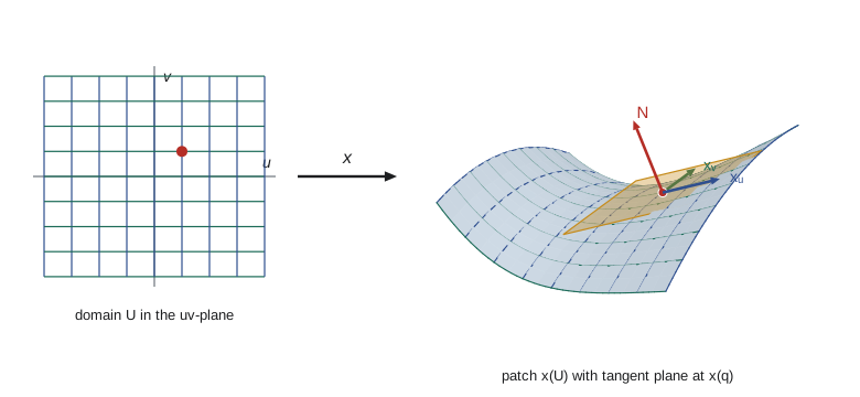
Such a map is a local parametrization, or coordinate patch, and \(V \cap S\) is a coordinate neighbourhood. Writing \(\mathbf{x}(u, v) = (x(u, v), y(u, v), z(u, v))\), the differential has as its columns the partial derivatives \(\mathbf{x}_u\) and \(\mathbf{x}_v\), so condition 3 says these two vectors are linearly independent, equivalently \(\mathbf{x}_u \times \mathbf{x}_v \ne 0\). This is the surface analogue of regularity for curves.

Each condition does a job. Smoothness lets us use calculus. The homeomorphism condition rules out sets that touch or cross themselves: a figure-eight-shaped tube, or a parametrized surface that passes through the same point twice, can satisfy conditions 1 and 3 and still fail to look like a single piece of plane at the crossing. Condition 3 rules out cusps and edges, and guarantees the tangent plane below. The definition is about the set \(S\), not about one particular map: different patches are allowed to overlap, and most surfaces need several.

Graphs

The simplest surfaces are graphs. If \(f : U \to \mathbb{R}\) is smooth on an open set \(U \subseteq \mathbb{R}^2\), its graph \(\{(u, v, f(u, v))\}\) is a regular surface covered by the single patch \(\mathbf{x}(u, v) = (u, v, f(u, v))\). It is smooth; it is a homeomorphism onto the graph because its inverse is the restriction of the projection \((x, y, z) \mapsto (x, y)\), which is continuous; and \(\mathbf{x}_u = (1, 0, f_u)\), \(\mathbf{x}_v = (0, 1, f_v)\) are independent because of their first two components. The paraboloid \(z = u^2 + v^2\) and the saddle \(z = u^2 - v^2\) are examples.

The unit sphere \(S^2 = \{x^2 + y^2 + z^2 = 1\}\) is not a graph, but it is covered by six graphs: the upper hemisphere \(z = \sqrt{1 - x^2 - y^2}\) over the open unit disc, the lower hemisphere \(z = -\sqrt{1 - x^2 - y^2}\), and four more in the \(x\) and \(y\) directions. Every point of the sphere has at least one nonzero coordinate and lies in the corresponding open hemisphere, so the six patches cover. This proves that the sphere is a regular surface.

Level sets

Most surfaces in practice are described by equations. A number \(c\) is a regular value of a smooth function \(F : \mathbb{R}^3 \to \mathbb{R}\) if \(\nabla F(p) \ne 0\) at every point of the level set \(F^{-1}(c)\).

Theorem. If \(c\) is a regular value of \(F\) and \(F^{-1}(c)\) is nonempty, then \(F^{-1}(c)\) is a regular surface.

Proof. Let \(p \in F^{-1}(c)\). Since \(\nabla F(p) \ne 0\), some partial derivative is nonzero; say \(F_z(p) \ne 0\). By the implicit function theorem there are open sets \(U \ni (p_1, p_2)\) and an open interval \(I \ni p_3\), and a smooth function \(g : U \to I\), such that for \((x, y, z) \in U \times I\), \(F(x, y, z) = c\) holds exactly when \(z = g(x, y)\). So with \(V = U \times I\), the set \(V \cap F^{-1}(c)\) is the graph of \(g\), which is covered by the patch \((x, y) \mapsto (x, y, g(x, y))\) satisfying all three conditions. The cases \(F_x(p) \ne 0\) and \(F_y(p) \ne 0\) are the same with the roles of the coordinates changed. \(\blacksquare\)

This theorem immediately gives the sphere again (\(F = x^2 + y^2 + z^2\), \(\nabla F = 2(x, y, z) \ne 0\) on \(F = 1\)), the ellipsoid \(x^2/a^2 + y^2/b^2 + z^2/c^2 = 1\), the hyperboloid of one sheet \(x^2 + y^2 - z^2 = 1\) and of two sheets \(x^2 + y^2 - z^2 = -1\), and the torus \(\big(\sqrt{x^2 + y^2} - R\big)^2 + z^2 = r^2\) with \(0 < r < R\). The cone \(x^2 + y^2 - z^2 = 0\) is not covered: \(0\) is not a regular value because \(\nabla F = 0\) at the origin. The cone is in fact not a regular surface at its tip, since removing the tip disconnects every small neighbourhood of it into two pieces, while removing a point from a disc leaves it connected.

Surfaces of revolution

Rotating a regular plane curve \((f(v), g(v))\), with \(f > 0\), about the \(z\)-axis sweeps out a surface of revolution, parametrized by

The curves \(u = \text{constant}\) are meridians, copies of the profile curve, and the curves \(v = \text{constant}\) are parallels, horizontal circles of radius \(f(v)\). The partial derivatives are \(\mathbf{x}_u = (-f\sin u, f\cos u, 0)\) and \(\mathbf{x}_v = (f'\cos u, f'\sin u, g')\), with \(|\mathbf{x}_u \times \mathbf{x}_v| = f\sqrt{f'^2 + g'^2} > 0\), so the map is regular. To get a homeomorphism we restrict \(u\) to an open interval of length \(2\pi\), such as \((0, 2\pi)\), which misses one meridian; a second patch with \(u \in (-\pi, \pi)\) covers it. With profile circle \((R + r\cos v, r\sin v)\) we get the torus; with \((\cosh v, v)\) the catenoid of lesson 8; with \((\cos v, \sin v)\) for \(-\pi/2 < v < \pi/2\) the sphere minus its poles.

Change of parameters

A point of a surface usually lies in several coordinate patches, and we want definitions such as the tangent plane or the curvature not to depend on which patch we use. The key fact is that the transition between two patches is smooth.

Theorem. Let \(\mathbf{x} : U \to S\) and \(\mathbf{y} : W \to S\) be local parametrizations whose images overlap in \(O\). Then the change of parameters \(h = \mathbf{x}^{-1} \circ \mathbf{y} : \mathbf{y}^{-1}(O) \to \mathbf{x}^{-1}(O)\) is a diffeomorphism.

Proof sketch. The map \(h\) is a homeomorphism as a composition of homeomorphisms; the issue is smoothness, since \(\mathbf{x}^{-1}\) is defined only on the surface and we do not yet know what it means to differentiate it. Fix \(q\) with \(\mathbf{x}(q) = p\). Because \(d\mathbf{x}_q\) is injective, some two rows of its Jacobian form an invertible matrix; say the \(x\) and \(y\) rows. Extend \(\mathbf{x}\) to a map of three variables, \(F(u, v, t) = \mathbf{x}(u, v) + (0, 0, t)\). Its Jacobian at \((q, 0)\) is invertible, so by the inverse function theorem \(F\) has a smooth inverse \(F^{-1}\) on a neighbourhood of \(p\) in \(\mathbb{R}^3\). On the surface, \(F^{-1}\) agrees with \(\mathbf{x}^{-1}\) followed by inclusion \((u, v) \mapsto (u, v, 0)\). So near \(\mathbf{y}^{-1}(p)\), \(h\) is the composition of the smooth maps \(\mathbf{y}\), \(F^{-1}\) and projection onto the first two coordinates, hence smooth. The same argument applies to \(h^{-1}\). \(\blacksquare\)

This theorem is what makes differential geometry of surfaces well defined. A function \(f : S \to \mathbb{R}\) is called smooth at \(p\) if \(f \circ \mathbf{x}\) is smooth near \(\mathbf{x}^{-1}(p)\) for some patch \(\mathbf{x}\); by the theorem, it is then smooth for every patch, because \(f \circ \mathbf{y} = (f \circ \mathbf{x}) \circ h\). Lesson 12 turns this observation into the definition of an abstract manifold, where there is no surrounding \(\mathbb{R}^3\) at all and smooth transition maps are assumed instead of proved.

The tangent plane

A tangent vector to \(S\) at \(p\) is the velocity \(\alpha'(0)\) of a smooth curve \(\alpha : (-\varepsilon, \varepsilon) \to S\) with \(\alpha(0) = p\). The set of all tangent vectors is the tangent plane \(T_pS\).

Theorem. If \(\mathbf{x}\) is a local parametrization with \(\mathbf{x}(q) = p\), then \(T_pS = d\mathbf{x}_q(\mathbb{R}^2)\), the two-dimensional subspace spanned by \(\mathbf{x}_u(q)\) and \(\mathbf{x}_v(q)\).

Proof. If \(w = (w_1, w_2) \in \mathbb{R}^2\), the curve \(\alpha(t) = \mathbf{x}(q + tw)\) lies on \(S\), and by the chain rule \(\alpha'(0) = w_1\mathbf{x}_u + w_2\mathbf{x}_v = d\mathbf{x}_q(w)\). So the image of \(d\mathbf{x}_q\) consists of tangent vectors. Conversely, let \(\alpha\) be a curve on \(S\) through \(p\). For small \(t\) it lies in the coordinate neighbourhood, and \(\beta = \mathbf{x}^{-1} \circ \alpha\) is a smooth curve in \(U\), by the change-of-parameters argument (the map \(F^{-1}\) above is smooth). Then \(\alpha = \mathbf{x} \circ \beta\) and \(\alpha'(0) = d\mathbf{x}_q(\beta'(0))\). Since \(d\mathbf{x}_q\) is injective its image is two-dimensional. \(\blacksquare\)

In coordinates, a tangent vector \(w = a\mathbf{x}_u + b\mathbf{x}_v\) corresponds to the pair \((a, b)\), and a curve \(\alpha(t) = \mathbf{x}(u(t), v(t))\) has velocity \(u'\mathbf{x}_u + v'\mathbf{x}_v\). The tangent plane does not depend on the patch, because it was defined by curves. For a level set \(F = c\), every curve \(\alpha\) on the surface satisfies \(F(\alpha(t)) = c\), so \(\nabla F(p) \cdot \alpha'(0) = 0\): the tangent plane is the orthogonal complement of the gradient,

For the unit sphere, \(T_pS = \{w : p \cdot w = 0\}\), the plane perpendicular to the radius, as expected.

Normals and orientation

At each point of a patch, the vector

is a unit normal: it is perpendicular to \(T_pS\) and has length 1. There are exactly two unit normals at each point, \(\pm N\). Under a change of parameters \(h\) with Jacobian determinant \(J\), the chain rule gives \(\mathbf{y}_{\bar u} \times \mathbf{y}_{\bar v} = J\,\mathbf{x}_u \times \mathbf{x}_v\), so the two patches define the same normal where \(J > 0\) and opposite normals where \(J < 0\). A surface is orientable if it can be covered by patches whose transition maps all have positive Jacobian, equivalently if there is a continuous unit normal field on all of \(S\). Level sets of regular values are always orientable, with \(N = \nabla F/|\nabla F|\). The Möbius strip is the standard example of a non-orientable surface: carrying a normal once around its centre line brings it back pointing the other way. Lesson 11 shows that orientability is needed to integrate curvature.

Computations

The program verifies regularity and normals for the torus with \(R = 2\), \(r = 1\) in three independent ways: from the cross product of the partial derivatives (computed by central differences), from the gradient of the defining function \(F = (\sqrt{x^2 + y^2} - 2)^2 + z^2\), and from the exact formula of the example. It then checks that the tangent vector of a curve on the torus lies in the tangent plane, and computes the Jacobian determinant of the change of parameters between two overlapping patches of the sphere: the latitude-longitude patch and the upper-hemisphere graph patch.

import math

R, r = 2.0, 1.0
def torus(u, v): return [(R + r*math.cos(v))*math.cos(u), (R + r*math.cos(v))*math.sin(u), r*math.sin(v)]
def F(p): return (math.hypot(p[0], p[1]) - R)**2 + p[2]**2
def cross(a, b): return [a[1]*b[2] - a[2]*b[1], a[2]*b[0] - a[0]*b[2], a[0]*b[1] - a[1]*b[0]]
def dot(a, b): return sum(x*y for x, y in zip(a, b))
def unit(a):
    n = math.sqrt(dot(a, a)); return [x / n for x in a]
h = 1e-5
def partials(X, u, v):
    xu = [(a - b) / (2*h) for a, b in zip(X(u + h, v), X(u - h, v))]
    xv = [(a - b) / (2*h) for a, b in zip(X(u, v + h), X(u, v - h))]
    return xu, xv

for (u, v) in [(0.3, 0.0), (1.0, 2.0), (2.5, math.pi)]:
    xu, xv = partials(torus, u, v)
    c = cross(xu, xv); N1 = unit(c)
    p = torus(u, v)
    grad = [(F([p[j] + (h if j == i else 0) for j in range(3)]) - F([p[j] - (h if j == i else 0) for j in range(3)])) / (2*h) for i in range(3)]
    N2 = unit(grad)
    N3 = [math.cos(u)*math.cos(v), math.sin(u)*math.cos(v), math.sin(v)]
    print(f"(u,v)=({u},{v:.3f}): |xu x xv|={math.sqrt(dot(c, c)):.6f} (exact {r*(R + r*math.cos(v)):.6f})"
          f"  N.grad-normal={dot(N1, N2):+.8f}  N.exact={dot(N1, N3):+.8f}")

# a curve on the torus: u = t, v = 3t (a (1,3) torus knot); its velocity lies in the tangent plane
t = 0.7
alpha = lambda t: torus(t, 3*t)
vel = [(a - b) / (2*h) for a, b in zip(alpha(t + h), alpha(t - h))]
xu, xv = partials(torus, t, 3*t)
print(f"velocity . normal = {dot(vel, unit(cross(xu, xv))):.2e}   velocity - (xu + 3 xv) = "
      f"{max(abs(a - (b + 3*c)) for a, b, c in zip(vel, xu, xv)):.2e}")

# change of parameters on the sphere: (lat, lon) -> (x, y) of the graph patch z = sqrt(1 - x^2 - y^2)
def hmap(phi, th): return [math.cos(phi)*math.cos(th), math.cos(phi)*math.sin(th)]
for phi in (0.3, 0.8, 1.4):
    th = 0.5
    a = [(p - q) / (2*h) for p, q in zip(hmap(phi + h, th), hmap(phi - h, th))]
    b = [(p - q) / (2*h) for p, q in zip(hmap(phi, th + h), hmap(phi, th - h))]
    J = a[0]*b[1] - a[1]*b[0]
    print(f"latitude {phi}: Jacobian of the transition = {J:+.6f}   exact -sin(phi)cos(phi) = {-math.sin(phi)*math.cos(phi):+.6f}")

(u,v)=(0.3,0.000): |xu x xv|=3.000000 (exact 3.000000)  N.grad-normal=+1.00000000  N.exact=+1.00000000
(u,v)=(1.0,2.000): |xu x xv|=1.583853 (exact 1.583853)  N.grad-normal=+1.00000000  N.exact=+1.00000000
(u,v)=(2.5,3.142): |xu x xv|=1.000000 (exact 1.000000)  N.grad-normal=+1.00000000  N.exact=+1.00000000
velocity . normal = -9.48e-11   velocity - (xu + 3 xv) = 5.22e-10
latitude 0.3: Jacobian of the transition = -0.282321   exact -sin(phi)cos(phi) = -0.282321
latitude 0.8: Jacobian of the transition = -0.499787   exact -sin(phi)cos(phi) = -0.499787
latitude 1.4: Jacobian of the transition = -0.167494   exact -sin(phi)cos(phi) = -0.167494

All three normals agree to eight digits, and \(|\mathbf{x}_u \times \mathbf{x}_v|\) matches \(r(R + r\cos v)\), which is largest on the outer equator (\(v = 0\)) and smallest on the inner equator (\(v = \pi\)). The velocity of the torus knot is \(\mathbf{x}_u + 3\mathbf{x}_v\), as the chain rule predicts, and is perpendicular to the normal. The transition Jacobian from latitude-longitude coordinates to the graph coordinates is \(-\sin\varphi\cos\varphi\), negative throughout the upper hemisphere: the two patches induce opposite orientations, and one of them must be composed with a reflection, say \(\theta \mapsto -\theta\), to belong to an oriented atlas. Its absolute value tends to 0 as the latitude approaches \(\pi/2\), where the latitude-longitude patch fails to be regular at the pole.