Capstone: smooth manifolds, Riemannian metrics and the road to general relativity

Gauss showed that the geometry of a surface can be done from the inside, using only the first fundamental form. Riemann, in his habilitation lecture of 10 June 1854, took the next step: if the inhabitants need only the metric, why should there be a surrounding space at all, and why only two dimensions? This capstone lesson builds the framework he envisioned. A smooth manifold is a space covered by coordinate charts with smooth transitions, and a Riemannian metric assigns an inner product to each tangent space. Lengths, geodesics, parallel transport and curvature carry over with the formulas of lessons 6 to 11 written in index notation. The lesson ends where the subject changed physics: Einstein's description of gravity as the curvature of a four-dimensional spacetime, analysed here through a surface you can draw, Flamm's paraboloid.

Smooth manifolds

A topological manifold of dimension \(n\) is a Hausdorff space with a countable basis of open sets in which every point has a neighbourhood homeomorphic to an open subset of \(\mathbb{R}^n\). A chart is such a homeomorphism \(\varphi : U \to \varphi(U) \subseteq \mathbb{R}^n\) from an open set \(U\) of the manifold; its components \(x^1, \dots, x^n\) are local coordinates. Two charts \((U, \varphi)\) and \((V, \psi)\) are smoothly compatible if the transition map

is smooth with smooth inverse. A smooth atlas is a collection of pairwise compatible charts covering the manifold, and a smooth manifold is a topological manifold together with a maximal smooth atlas. This reverses the logic of lesson 5. There, surfaces lived in \(\mathbb{R}^3\) and we proved that transition maps are smooth; here smoothness of transitions is the definition, and no ambient space is needed. The definition was formulated by Hermann Weyl in 1913 for surfaces and by Hassler Whitney and others in the 1930s in general.

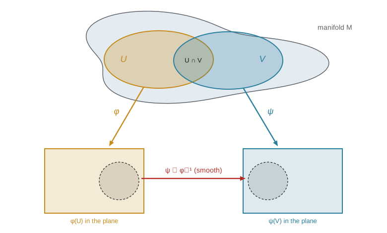
Examples abound. Every regular surface is a two-dimensional manifold, with the inverses of its local parametrizations as charts. The sphere \(S^n \subset \mathbb{R}^{n+1}\) is covered by two stereographic charts, from the north and south poles, whose transition map is the inversion \(y \mapsto y/|y|^2\) on \(\mathbb{R}^n \setminus \{0\}\). The flat torus \(\mathbb{R}^2/\mathbb{Z}^2\), the plane with points identified when they differ by integer vectors, is a manifold whose charts are small squares, and it is not given as a subset of anything. The real projective plane, the set of lines through the origin in \(\mathbb{R}^3\), is a compact non-orientable two-manifold that cannot be embedded in \(\mathbb{R}^3\) at all. More generally, if \(F : \mathbb{R}^{n+k} \to \mathbb{R}^k\) is smooth and \(c\) is a regular value, the level set \(F^{-1}(c)\) is an \(n\)-manifold by the implicit function theorem of MATH-341, as lesson 5 proved for \(n = 2\), \(k = 1\). The group of rotations \(SO(3)\), the configuration space of a rigid body, is a three-manifold of this kind.

A function \(f\) on a manifold is smooth if \(f \circ \varphi^{-1}\) is smooth for every chart, and maps between manifolds are smooth if they are smooth in charts. A tangent vector at \(p\) can be defined, as in lesson 5, as an equivalence class of curves through \(p\) with the same velocity in one, hence every, chart; equivalently, as the directional derivative operator it defines on smooth functions. In a chart the tangent space \(T_pM\) has the basis \(\partial_1, \dots, \partial_n\) of coordinate directions, and a vector is \(w = w^i\partial_i\), using the summation convention: a repeated upper and lower index is summed from 1 to \(n\). Whitney proved in 1936 that every smooth \(n\)-manifold can be embedded in \(\mathbb{R}^{2n+1}\), and in 1944 improved this to \(\mathbb{R}^{2n}\), so abstract manifolds are no more general than submanifolds of Euclidean space; but the abstract viewpoint is the natural one, because the embedding carries no meaning.

Riemannian metrics

A Riemannian metric on a smooth manifold \(M\) is a choice of inner product \(g_p\) on each tangent space \(T_pM\), varying smoothly with \(p\). In a chart it is given by the symmetric positive definite matrix of functions \(g_{ij} = g(\partial_i, \partial_j)\), and one writes

For a surface in \(\mathbb{R}^3\) with the induced metric, \(g_{11} = E\), \(g_{12} = F\), \(g_{22} = G\): the first fundamental form is the prototype. But now metrics can be prescribed freely. The Poincaré half-plane \(\frac{dx^2 + dy^2}{y^2}\) of lesson 9, the flat torus with \(dx^2 + dy^2\), and the round metric on \(S^n\) are examples. Lengths of curves, \(L = \int\sqrt{g_{ij}\dot x^i\dot x^j}\,dt\), angles and volumes, with volume element \(\sqrt{\det g}\,dx^1 \cdots dx^n\), are defined exactly as in lesson 6. John Nash proved in 1956 that every Riemannian manifold can be isometrically embedded in some Euclidean space, of dimension much larger than \(n\), so the abstract metric is always the first fundamental form of something; Hilbert's theorem from lesson 9 shows that the dimension cannot always be kept small.

Connections, geodesics and curvature

The Christoffel symbols of lesson 9 generalize directly. The Levi-Civita connection, named for Tullio Levi-Civita, who introduced parallel transport in 1917, is determined by the metric through

where \(g^{kl}\) is the inverse matrix. In two dimensions these are exactly the solutions of the linear systems in the lemma of lesson 9. The covariant derivative of a vector field \(w = w^k\partial_k\) along a curve \(x(t)\) is \(\frac{Dw}{dt} = \big(\dot w^k + \Gamma^k_{ij}\dot x^i w^j\big)\partial_k\), parallel transport means \(Dw/dt = 0\), and geodesics satisfy

the equations of lesson 10 in index form. Geodesics are critical points of length and are locally length-minimizing. Curvature in higher dimensions measures the failure of parallel transport around small loops to return vectors to themselves, which lesson 11 identified with \(K\) for surfaces. Covariant derivatives along different coordinate directions do not commute, and the commutator defines the Riemann curvature tensor,

introduced by Riemann in an 1861 essay and systematized by Ricci and Levi-Civita in their 1900 paper on the absolute differential calculus. For each two-dimensional plane \(\sigma \subset T_pM\) spanned by \(v, w\), the sectional curvature \(K(\sigma) = \frac{R(v, w, w, v)}{|v|^2|w|^2 - \langle v, w \rangle^2}\) is the Gaussian curvature at \(p\) of the surface swept out by geodesics tangent to \(\sigma\). In dimension 2 there is only one plane, and \(R_{1212} = K\,(EG - F^2)\): the Riemann tensor is the Theorema Egregium generalized. Contracting gives the Ricci tensor \(R_{ij} = R^k{}_{ikj}\), which measures how volumes of small geodesic balls differ from Euclidean ones, and the scalar curvature \(R = g^{ij}R_{ij}\), equal to \(2K\) for a surface.

Global theorems generalize too, often in deep ways. The Bonnet–Myers theorem says a complete manifold with Ricci curvature bounded below by a positive constant is compact. The uniformization theorem of Koebe and Poincaré (1907) says every surface carries a metric of constant curvature \(1\), \(0\) or \(-1\), with the sign fixed by the Euler characteristic, in accord with Gauss–Bonnet. Richard Hamilton introduced the Ricci flow \(\partial_t g_{ij} = -2R_{ij}\) in 1982, a heat equation for metrics that smooths out curvature, and Grigori Perelman used it in 2002 and 2003 to prove the Poincaré conjecture and Thurston's geometrization conjecture: every closed simply connected three-manifold is a three-sphere.

Spacetime and gravity

In 1907 Albert Einstein noticed that a person falling freely does not feel their own weight. Gravity, unlike every other force, accelerates all bodies equally, so locally it can be transformed away by choosing a freely falling frame, just as a curved surface is locally indistinguishable from its tangent plane. After eight years of work, much of it learning Riemannian geometry with the help of his friend Marcel Grossmann, Einstein presented the field equations of general relativity in November 1915. In the theory, spacetime is a four-dimensional manifold with a metric \(g_{\mu\nu}\) that is not positive definite but has signature \((-, +, +, +)\), a Lorentzian metric. Freely falling bodies follow timelike geodesics, light follows null geodesics, and matter curves spacetime according to

where \(T_{\mu\nu}\) is the stress-energy tensor of matter and \(G\) is Newton's constant. John Wheeler's summary is often quoted: spacetime tells matter how to move, and matter tells spacetime how to curve. All of the machinery of this course reappears: the Christoffel symbols of \(g_{\mu\nu}\) play the role of the gravitational field, the geodesic equation replaces Newton's second law, and tidal forces, which stretch a falling body, are the geodesic deviation of the Jacobi equation, governed by curvature.

Karl Schwarzschild found in 1916 the exact solution outside a spherical mass \(M\). With \(r_s = 2GM/c^2\), the Schwarzschild radius, its metric is

Its predictions have been confirmed again and again. The orbit of Mercury precesses by about 43 arcseconds per century more than Newtonian theory predicts, which Einstein computed in November 1915. Starlight grazing the Sun is deflected by about 1.75 arcseconds, measured by Arthur Eddington's and Andrew Crommelin's expeditions during the eclipse of 29 May 1919. Clocks run slower deeper in a gravitational well, an effect the Global Positioning System must correct for. Gravitational waves, ripples in the metric itself, were detected by the LIGO observatories on 14 September 2015, from two black holes merging over a billion light years away, and the Event Horizon Telescope imaged the shadow of the black hole in the galaxy M87 in 2019.

Capstone analysis: Flamm's paraboloid

The full Schwarzschild metric is four-dimensional, but its spatial geometry in the equatorial plane is a surface we can study with this course's tools. Fix a time \(t\) and set \(\theta = \pi/2\). The metric induced on this slice is

Ludwig Flamm showed in 1916 that this is the first fundamental form of a surface of revolution in \(\mathbb{R}^3\). Look for a profile \(z = z(r)\) rotated about the \(z\)-axis: the induced metric is \((1 + z'(r)^2)\,dr^2 + r^2\,d\phi^2\), so we need \(1 + z'^2 = \frac{1}{1 - r_s/r}\), that is \(z'^2 = \frac{r_s}{r - r_s}\). Integrating, \(z = 2\sqrt{r_s(r - r_s)}\), equivalently \(r = r_s + \frac{z^2}{4r_s}\): a paraboloid of revolution lying on its side, with its throat, a circle of radius \(r_s\), at \(z = 0\). This is the embedding diagram familiar from popular pictures of black holes. It represents only the spatial geometry at one instant, not the motion of particles, which needs the time part of the metric.

Curvature. The metric is orthogonal with \(E = (1 - r_s/r)^{-1}\) and \(G = r^2\), depending only on \(u = r\). Using lesson 9's orthogonal formula, with \(\sqrt{EG} = r(1 - r_s/r)^{-1/2}\) and \(G_u = 2r\),

The spatial slice is negatively curved, most strongly at the throat, where \(K = -1/(2r_s^2)\), and it flattens out like \(r^{-3}\) far away, the same falloff as the tidal acceleration in Newtonian gravity. The total curvature outside radius \(r_0\) is \(\int_0^{2\pi}\int_{r_0}^\infty K\sqrt{EG}\,dr\,d\phi = -2\pi\big(1 - \sqrt{1 - r_s/r_0}\big)\), which tends to \(-2\pi\) at the throat. By local Gauss–Bonnet applied to the annulus between \(r_0\) and a large radius, this equals the turning of the boundary circles, which one can check: the circle \(r = r_0\) has geodesic curvature \(\sqrt{1 - r_s/r_0}/r_0\), slightly less than in flat space.

Circumference and radius. On this surface a circle of coordinate radius \(r\) has circumference exactly \(2\pi r\), but the proper radial distance between two circles exceeds the difference of their \(r\) values: \(\int_{r_1}^{r_2}\frac{dr}{\sqrt{1 - r_s/r}} > r_2 - r_1\). Space near a mass is stretched radially, exactly the geometry of the paraboloid, whose radial lines climb up the throat. For the Sun, \(r_s \approx 2.95\) km, and the effect at the solar surface, radius about 696,000 km, is a fractional stretch of about \(2 \times 10^{-6}\): small, but enough, together with the time part of the metric, to produce the deflection of starlight.

Geodesics on the slice. Flamm's paraboloid is a surface of revolution, so Clairaut's relation of lesson 10 applies: along a geodesic, \(r\cos\psi\) is constant. A geodesic coming in from far away with impact parameter \(b\) (its distance of closest approach in the absence of curvature) has \(r\cos\psi = b\) and turns back at \(r_{\min} = b\), where \(\psi = 0\); but it is deflected, bending around the throat, because the surface is negatively curved. These spatial geodesics are not the paths of light, which also feel the time part of the metric, and in fact the spatial curvature accounts for exactly half of the 1.75 arcsecond deflection, the other half coming from the time component. Einstein's first, 1911, calculation used only the time part and predicted 0.87 arcseconds, half the correct value, an error his 1915 theory corrected before any measurement was made.

Computing with the capstone model

The program does five things. It computes the Christoffel symbols of a general metric numerically from \(g_{ij}\) by the index formula and checks them against the exact symbols of Flamm's metric. It computes \(K\) of Flamm's paraboloid three ways: from the metric by the orthogonal formula, from the embedded paraboloid in \(\mathbb{R}^3\) by \((eg - f^2)/(EG - F^2)\), and from the closed form \(-r_s/(2r^3)\). It integrates a geodesic on the paraboloid to measure the spatial bending of a path that passes the throat. And it evaluates three classic predictions of general relativity from their textbook formulas with physical constants: the extra precession of Mercury, the deflection of starlight by the Sun, and the daily clock correction for GPS satellites.

import math

def christoffel(g, x, h=1e-5):
    """Gamma^k_ij = 1/2 g^kl (d_i g_jl + d_j g_il - d_l g_ij) for a 2 x 2 metric g(x) by central differences."""
    n = 2
    G = g(x)
    det = G[0][0]*G[1][1] - G[0][1]*G[1][0]
    inv = [[G[1][1]/det, -G[0][1]/det], [-G[1][0]/det, G[0][0]/det]]
    dg = []
    for l in range(n):
        xp = list(x); xm = list(x); xp[l] += h; xm[l] -= h
        A, B = g(xp), g(xm)
        dg.append([[(A[i][j] - B[i][j])/(2*h) for j in range(n)] for i in range(n)])
    return [[[sum(0.5*inv[k][l]*(dg[i][j][l] + dg[j][i][l] - dg[l][i][j]) for l in range(n))
              for j in range(n)] for i in range(n)] for k in range(n)]

rs = 1.0
flamm = lambda x: [[1/(1 - rs/x[0]), 0.0], [0.0, x[0]**2]]          # coordinates (r, phi)
r0 = 1.6
Gam = christoffel(flamm, [r0, 0.3])
exact = {"G^r_rr": -rs/(2*r0*r0*(1 - rs/r0)), "G^r_pp": -(r0 - rs), "G^p_rp": 1/r0}
print(f"Gamma^r_rr {Gam[0][0][0]:+.6f} (exact {exact['G^r_rr']:+.6f})  Gamma^r_pp {Gam[0][1][1]:+.6f} (exact {exact['G^r_pp']:+.6f})"
      f"  Gamma^p_rp {Gam[1][0][1]:+.6f} (exact {exact['G^p_rp']:+.6f})")

# curvature of Flamm's paraboloid three ways
def K_metric(r, h=1e-4):
    sq = lambda r: math.sqrt(r*r/(1 - rs/r))                       # sqrt(EG)
    q = lambda r: 2*r/sq(r)                                          # G_u / sqrt(EG)
    return -1/(2*sq(r)) * (q(r + h) - q(r - h))/(2*h)
def K_embedded(r, h=1e-4):
    X = lambda r, p: [r*math.cos(p), r*math.sin(p), 2*math.sqrt(rs*(r - rs))]
    P = lambda i, j: X(r + i*h, 0.2 + j*h)
    xu = [(a - b)/(2*h) for a, b in zip(P(1, 0), P(-1, 0))]; xv = [(a - b)/(2*h) for a, b in zip(P(0, 1), P(0, -1))]
    xuu = [(a - 2*m + b)/h**2 for a, m, b in zip(P(1, 0), P(0, 0), P(-1, 0))]
    xvv = [(a - 2*m + b)/h**2 for a, m, b in zip(P(0, 1), P(0, 0), P(0, -1))]
    xuv = [(a - b - c + d)/(4*h*h) for a, b, c, d in zip(P(1, 1), P(1, -1), P(-1, 1), P(-1, -1))]
    dot = lambda a, b: sum(x*y for x, y in zip(a, b))
    n = [xu[1]*xv[2] - xu[2]*xv[1], xu[2]*xv[0] - xu[0]*xv[2], xu[0]*xv[1] - xu[1]*xv[0]]
    W = math.sqrt(dot(n, n)); N = [x/W for x in n]
    return (dot(N, xuu)*dot(N, xvv) - dot(N, xuv)**2) / W**2
for r in (1.2, 2.0, 5.0):
    print(f"r = {r}: K from metric {K_metric(r):+.6f}, from embedding {K_embedded(r):+.6f}, closed form {-rs/(2*r**3):+.6f}")

# a geodesic on the slice passing the throat: integrate in (r, phi), start far out heading inward with impact parameter b
def rhs(y):
    r, p, dr, dp = y
    Gr_rr, Gr_pp, Gp_rp = -rs/(2*r*r*(1 - rs/r)), -(r - rs), 1/r
    return [dr, dp, -(Gr_rr*dr*dr + Gr_pp*dp*dp), -2*Gp_rp*dr*dp]
b, rstart = 3.0, 200.0
dp0 = b / rstart**2                                                  # r^2 phi' = b (Clairaut, unit speed)
dr0 = -math.sqrt((1 - rs/rstart) * (1 - b*b/rstart**2))
y, h, rmin = [rstart, 0.0, dr0, dp0], 0.02, rstart
while True:
    k1 = rhs(y); k2 = rhs([a + h/2*c for a, c in zip(y, k1)]); k3 = rhs([a + h/2*c for a, c in zip(y, k2)]); k4 = rhs([a + h*c for a, c in zip(y, k3)])
    y = [a + h/6*(c + 2*d + 2*e + f) for a, c, d, e, f in zip(y, k1, k2, k3, k4)]
    rmin = min(rmin, y[0])
    if y[0] > rstart: break
print(f"spatial geodesic with b = {b}: closest r = {rmin:.4f}, total change of angle {math.degrees(y[1]):.3f} deg "
      f"(straight line: {math.degrees(2*math.asin(1) - 2*math.asin(b/rstart)):.3f} deg)")

# three classic predictions of general relativity
G, c = 6.674e-11, 2.998e8
Msun, Rsun = 1.989e30, 6.957e8
a_merc, e_merc, T_merc = 5.791e10, 0.2056, 87.969                   # semi-major axis (m), eccentricity, period (days)
dphi = 6*math.pi*G*Msun / (c*c*a_merc*(1 - e_merc**2))              # radians per orbit
per_century = dphi * (36525 / T_merc) * 180/math.pi * 3600
print(f"Mercury: extra perihelion precession {per_century:.1f} arcseconds per century")
defl = 4*G*Msun / (c*c*Rsun) * 180/math.pi * 3600
print(f"starlight grazing the Sun: deflection {defl:.3f} arcseconds (Einstein 1911 value {defl/2:.3f})")
Mearth, Rearth, r_gps = 5.972e24, 6.371e6, 2.6560e7
v = math.sqrt(G*Mearth / r_gps)
grav = G*Mearth/(c*c) * (1/Rearth - 1/r_gps) * 86400e6               # microseconds per day, clocks aloft run fast
vel = -v*v/(2*c*c) * 86400e6                                         # orbital speed makes them run slow
print(f"GPS clocks: gravitational +{grav:.1f} us/day, velocity {vel:.1f} us/day, net {grav + vel:+.1f} us/day")
print(f"Schwarzschild radius of the Sun: {2*G*Msun/(c*c)/1000:.3f} km")

Gamma^r_rr -0.520833 (exact -0.520833)  Gamma^r_pp -0.600000 (exact -0.600000)  Gamma^p_rp +0.625000 (exact +0.625000)
r = 1.2: K from metric -0.289352, from embedding -0.289352, closed form -0.289352
r = 2.0: K from metric -0.062500, from embedding -0.062500, closed form -0.062500
r = 5.0: K from metric -0.004000, from embedding -0.004000, closed form -0.004000
spatial geodesic with b = 3.0: closest r = 3.0000, total change of angle 202.326 deg (straight line: 178.281 deg)
Mercury: extra perihelion precession 43.0 arcseconds per century
starlight grazing the Sun: deflection 1.752 arcseconds (Einstein 1911 value 0.876)
GPS clocks: gravitational +45.7 us/day, velocity -7.2 us/day, net +38.5 us/day
Schwarzschild radius of the Sun: 2.954 km

The numerical Christoffel symbols agree with the exact ones \(\Gamma^r_{rr} = -\frac{r_s}{2r^2(1 - r_s/r)}\), \(\Gamma^r_{\phi\phi} = -(r - r_s)\) and \(\Gamma^\phi_{r\phi} = 1/r\). The curvature of Flamm's paraboloid computed intrinsically from the metric, extrinsically from the paraboloid in space, and from the closed form \(-r_s/(2r^3)\) agree to six digits at every radius, a final demonstration of the Theorema Egregium. The spatial geodesic with impact parameter \(b = 3r_s\) turns back exactly at \(r = 3r_s\), as Clairaut's relation predicts, and sweeps through about 202 degrees instead of the 178 degrees of a straight line through the same far-away points: the negatively curved throat bends paths around it. The three physical predictions come out as the classic numbers: 43.0 arcseconds per century for Mercury, 1.75 arcseconds for light grazing the Sun, twice Einstein's 1911 value, and a net gain of about 38.5 microseconds per day for GPS satellite clocks, a drift that would accumulate to a positioning error of roughly 11 km per day if the system ignored the curvature of spacetime.

Where to go next

This course has followed the classical path from curves to surfaces to Riemannian geometry. Each step opens further subjects. Differential topology studies smooth manifolds without metrics, with tools such as transversality and degree theory; the Poincaré–Hopf theorem of lesson 11 is a first example. Riemannian geometry proper studies comparison theorems, in which curvature bounds control distances, volumes and topology. Lie groups, manifolds that are also groups such as the rotation group \(SO(3)\), unite geometry with algebra and underlie the symmetries of physics. Minimal surfaces and geometric flows such as the mean curvature flow and the Ricci flow connect geometry with partial differential equations. MATH-441 and MATH-445 supply the measure theory and functional analysis these subjects use, MATH-447 the topology, and the physics of curved spacetime is the natural continuation of the capstone.