Why differential geometry: measuring shape from the inside

Differential geometry studies shape with the tools of calculus. A curve bends and twists; a surface curves one way in one direction and another way in another; a space may be curved in ways that no outside observer is needed to detect. The subject asks how to measure these things, which measurements depend on how a shape sits in space and which belong to the shape itself, and what local measurements can tell us about global structure. This first lesson sets out the questions the course answers, previews the main theorems, and fixes the background from MATH-341 that we will use: derivatives as linear maps, the inverse and implicit function theorems, and a little linear algebra.

Two kinds of geometric information

Picture an ant living on a sheet of paper. It can measure distances by pacing along the paper, angles by comparing directions, and areas by counting tiles. Now roll the paper into a cylinder. To us, standing outside, the sheet is visibly curved. To the ant nothing has changed: every path keeps its length, every angle its size, every region its area. Rolling is an example of an isometry, a map that preserves lengths of curves on the surface. Any quantity the ant can compute is unchanged by isometries. We call such quantities intrinsic. Quantities that depend on how the surface sits in space, such as the direction its normal points or how sharply it bends away from a tangent plane, are extrinsic.

The cylinder is extrinsically curved but intrinsically flat. A sphere is different. No piece of a sphere can be flattened onto a plane without stretching or tearing, which is why every flat map of the Earth distorts something: the Mercator projection preserves angles but inflates areas near the poles, and equal-area projections distort shapes. Gauss proved in 1827 that this is not a failure of cartographers but a theorem. He found a number, the Gaussian curvature \(K\), that the ant can compute from measurements on the surface alone. For a plane \(K = 0\), for a cylinder \(K = 0\), and for a sphere of radius \(R\) the curvature is \(K = 1/R^2\) everywhere. Since isometries preserve \(K\), no isometry carries a piece of the sphere to a piece of the plane. Gauss was so pleased by this discovery that he named it the Theorema Egregium, the remarkable theorem. Lesson 9 proves it.

Angles of a triangle on a sphere

An ant on a sphere can detect curvature without any formula. Walk from the north pole down a meridian to the equator, turn left through a right angle, walk a quarter of the way around the equator, turn left again through a right angle, and walk back up a meridian to the pole. The path is a triangle whose sides are arcs of great circles, the straightest possible paths on the sphere. Each of its three angles is a right angle, so the angle sum is \(270^\circ\), not \(180^\circ\). On a sphere of radius \(R\) this triangle covers one eighth of the surface, an area of \(\frac{1}{8} \cdot 4\pi R^2 = \frac{\pi R^2}{2}\).

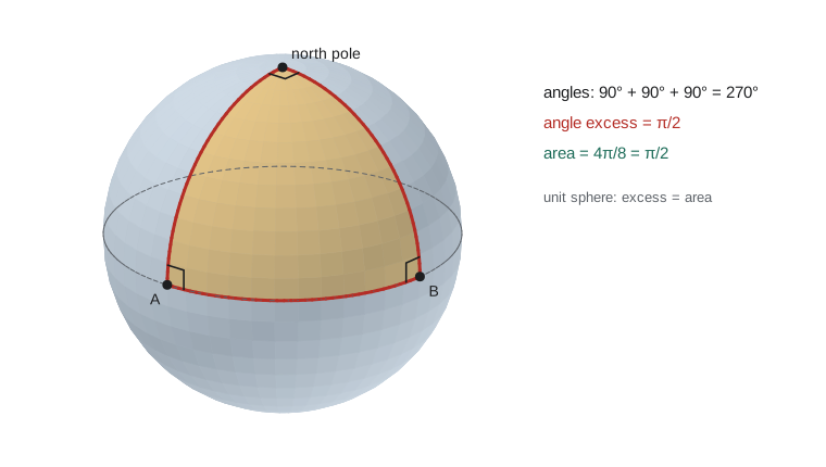
The angle excess, the amount by which the angle sum exceeds \(\pi\), is \(\frac{3\pi}{2} - \pi = \frac{\pi}{2}\). Divide the area by \(R^2\) and you also get \(\frac{\pi}{2}\). This is no coincidence. Thomas Harriot found in 1603, and Albert Girard published in 1629, that for any triangle on a sphere whose sides are great-circle arcs, the excess equals the area divided by \(R^2\). In the language of this course, the angle excess equals the integral of the Gaussian curvature over the triangle. Gauss proved the analogous statement for geodesic triangles on any surface, and Pierre Ossian Bonnet extended it in 1848 to regions bounded by arbitrary curves. The Gauss–Bonnet theorem of lesson 11 links local curvature, which is a derivative, to global topology, which is a count of holes, and it is the climax of the classical theory.

Curves first

Before surfaces come curves, where the ideas are simpler and the formulas are complete. A curve in space is described by a map \(\alpha : I \to \mathbb{R}^3\) from an interval. Its velocity \(\alpha'(t)\) points along the curve, and its speed \(|\alpha'(t)|\) says how fast we trace it. The same set of points can be traced at many speeds, so the geometric content of a curve is what survives a change of parameter. Lesson 2 shows that arc length gives a canonical parameter. Lesson 3 then defines two numbers at each point: the curvature \(\kappa\), which measures how fast the direction turns, and the torsion \(\tau\), which measures how fast the curve leaves its plane of bending. The fundamental theorem of curves says that \(\kappa\) and \(\tau\), given as functions of arc length, determine the curve up to a rigid motion. For curves, then, the local theory is completely solved by two functions.

Lesson 4 turns to global questions about closed plane curves. A closed curve has a total amount of turning, which must be a whole number of full turns; for a simple closed curve it is exactly one turn, a result of Heinz Hopf. Every simple closed convex curve has at least four points where the curvature has a local maximum or minimum, a theorem first proved by Syamadas Mukhopadhyaya in 1909. And among all closed curves of a given length, the circle encloses the most area, the isoperimetric inequality that the ancient Greeks knew and that was finally proved rigorously in the nineteenth century.

Then surfaces

A surface is a set in \(\mathbb{R}^3\) that looks locally like a piece of the plane, bent smoothly. Lesson 5 makes this precise with parametrizations \(\mathbf{x}(u, v)\) whose partial derivatives are linearly independent, and builds the tangent plane at each point. Lesson 6 introduces the first fundamental form, the dot product restricted to tangent planes, which lets the ant compute lengths, angles and areas from three functions \(E\), \(F\), \(G\). Lesson 7 studies how the unit normal turns as we move on the surface, packaged as the Gauss map and the second fundamental form, and lesson 8 extracts from it the principal curvatures, the Gaussian curvature \(K\) and the mean curvature \(H\). Surfaces with \(H = 0\) everywhere are minimal surfaces, the shapes of soap films.

With the machinery in place, lesson 9 proves the Theorema Egregium by expressing \(K\) entirely in terms of \(E\), \(F\), \(G\) and their derivatives. Lesson 10 asks what straight lines are on a curved surface. The answer, geodesics, comes from a derivative that the ant can compute, the covariant derivative, and lesson 10 shows how carrying a vector along a closed loop without turning it can still rotate it, an effect called holonomy that measures curvature. Lesson 11 proves Gauss–Bonnet, and lesson 12 lifts everything off \(\mathbb{R}^3\): a smooth manifold is a space covered by coordinate charts, a Riemannian metric is a first fundamental form defined without an ambient space, and Einstein's general relativity describes gravity as the curvature of a four-dimensional manifold.

What we use from analysis

This course relies on the multivariable calculus developed in MATH-341. A map \(f : U \to \mathbb{R}^m\) on an open set \(U \subseteq \mathbb{R}^n\) is differentiable at \(p\) if there is a linear map \(df_p\) with

and its matrix is the Jacobian of partial derivatives. We call \(f\) smooth if all partial derivatives of all orders exist and are continuous. The chain rule \(d(g \circ f)_p = dg_{f(p)} \circ df_p\) will be used constantly, usually in the form of differentiating along a curve: if \(\alpha(t)\) is a curve in \(U\), then \(\frac{d}{dt} f(\alpha(t)) = df_{\alpha(t)}(\alpha'(t))\). The inverse function theorem says that if \(df_p\) is invertible then \(f\) has a smooth local inverse near \(p\). The implicit function theorem says that if \(F : \mathbb{R}^3 \to \mathbb{R}\) is smooth with \(F(p) = 0\) and \(\nabla F(p) \ne 0\), then near \(p\) the set \(F = 0\) is the graph of a smooth function of two of the coordinates. Both theorems are the analytic engine behind the definitions of lesson 5.

From linear algebra we need the dot and cross products in \(\mathbb{R}^3\), orthonormal bases, the determinant as signed volume, and the spectral theorem: a symmetric linear map on a two-dimensional inner product space has an orthonormal basis of eigenvectors with real eigenvalues. That theorem is what produces the principal curvatures and principal directions of lesson 8.

Two identities about the cross product and dot product will be used often enough to record them now. For vectors \(a, b, c\) in \(\mathbb{R}^3\),

The second, sometimes called Lagrange's identity, says that the area of the parallelogram spanned by \(a\) and \(b\) is \(\sqrt{|a|^2|b|^2 - (a \cdot b)^2}\). In lesson 6 it becomes the formula \(\sqrt{EG - F^2}\) for the area element of a surface. Differentiating products also follows the usual rules: if \(a(t)\) and \(b(t)\) are differentiable vector functions, then \((a \cdot b)' = a' \cdot b + a \cdot b'\) and \((a \times b)' = a' \times b + a \times b'\), with the order of the cross product preserved.

A first computation

Many questions in this course can be checked numerically, and every lesson includes a short program using only Python's standard library. The first one measures the angle excess of geodesic triangles on the unit sphere. It places three points on the sphere, computes the angle at each vertex between the great-circle arcs meeting there, and compares the excess with the area. The area is computed independently by the formula of Van Oosterom and Strackee, which gives the solid angle of a triangle as seen from the centre. Agreement between the two is the Harriot–Girard theorem in action.

import math

def sub(a, b): return [a[i] - b[i] for i in range(3)]
def dot(a, b): return sum(a[i] * b[i] for i in range(3))
def cross(a, b): return [a[1]*b[2] - a[2]*b[1], a[2]*b[0] - a[0]*b[2], a[0]*b[1] - a[1]*b[0]]
def unit(a):
    n = math.sqrt(dot(a, a)); return [x / n for x in a]

def sph(lat, lon):
    la, lo = math.radians(lat), math.radians(lon)
    return [math.cos(la) * math.cos(lo), math.cos(la) * math.sin(lo), math.sin(la)]

def angle_at(p, q, r):
    """Angle at vertex p between the great-circle arcs to q and to r."""
    tq = unit(sub(q, [dot(p, q) * x for x in p]))   # tangent direction toward q
    tr = unit(sub(r, [dot(p, r) * x for x in p]))
    return math.acos(max(-1.0, min(1.0, dot(tq, tr))))

def area(a, b, c):
    """Solid angle of the triangle (Van Oosterom and Strackee, 1983)."""
    num = abs(dot(a, cross(b, c)))
    den = 1 + dot(a, b) + dot(b, c) + dot(c, a)
    return 2 * math.atan2(num, den)

tris = {"octant": (sph(90, 0), sph(0, 0), sph(0, 90)),
        "small":  (sph(10, 0), sph(0, 0), sph(0, 10)),
        "large":  (sph(60, 0), sph(-20, -40), sph(-10, 70))}
for name, (a, b, c) in tris.items():
    angs = [angle_at(a, b, c), angle_at(b, c, a), angle_at(c, a, b)]
    excess = sum(angs) - math.pi
    print(f"{name:7s} angles (deg) " + ", ".join(f"{math.degrees(t):7.3f}" for t in angs)
          + f"   excess {excess:.6f}   area {area(a, b, c):.6f}")

octant  angles (deg)  90.000,  90.000,  90.000   excess 1.570796   area 1.570796
small   angles (deg)  45.439,  90.000,  45.439   excess 0.015308   area 0.015308
large   angles (deg) 105.001,  87.955,  85.943   excess 1.726114   area 1.726114

The octant has three right angles and excess \(\pi/2 \approx 1.570796\). The small triangle, with sides of about ten degrees, has angles summing to only slightly more than \(180^\circ\): small regions of a sphere are nearly flat, which is why surveyors measuring a field can use plane geometry. During his survey of the Kingdom of Hanover in the 1820s, Gauss measured a large triangle formed by three mountain peaks, the Brocken, the Hoher Hagen and the Inselsberg. A popular story holds that he was testing whether physical space itself is curved; whatever his motive, the angle sum agreed with flat geometry to within his measurement errors. A century later Einstein showed that space and time are curved by mass, though far too slightly for a surveying triangle to detect.

Local and global

A recurring theme is the passage from local to global. Curvature is defined by derivatives at a point, so it is local: it depends only on the shape near that point. Topological properties such as being connected, being closed and bounded, or having a certain number of holes are global. The deepest theorems of differential geometry say that local measurements constrain global structure. The total curvature of a simple closed plane curve is \(2\pi\). The total Gaussian curvature of any closed surface equals \(2\pi\) times its Euler characteristic, so a sphere of any shape, however dented, has total curvature \(4\pi\), and a doughnut has total curvature zero. A compact surface in \(\mathbb{R}^3\) must have a point of positive curvature, as lesson 8 shows. These results reward the effort of setting up the local theory carefully.

Each lesson develops definitions, proves the main theorems, works examples by hand and checks them with code. The proofs are the point: the formulas of differential geometry are easy to misremember and hard to misprove. When a computation can be done in two ways, for instance by a formula and by a numerical approximation, doing both catches errors and builds intuition.

A brief history

The subject began with curves. Christiaan Huygens studied the curvature of curves in the 1670s while designing pendulum clocks, and Newton and Leibniz gave formulas for the radius of the osculating circle. Leonhard Euler, in 1760, studied how the curvature of a surface varies with direction and found that there are always two extreme directions at right angles, the principal directions of lesson 8. Gaspard Monge, teaching at the École Polytechnique around 1800, systematized the geometry of surfaces in space, and Jean Frenet in 1847 and Joseph Serret in 1851 independently found the moving frame of lesson 3. Carl Friedrich Gauss's 1827 memoir Disquisitiones generales circa superficies curvas founded the intrinsic geometry of surfaces. Bernhard Riemann's 1854 habilitation lecture extended intrinsic geometry to any number of dimensions, and his ideas, developed by Elwin Christoffel, Gregorio Ricci-Curbastro and Tullio Levi-Civita, became the language in which Einstein wrote general relativity in 1915.