
MATH-241 · Lesson 8 of 12 · 23 min
Continuity and the intermediate value theorem
A continuous function is one whose graph can be drawn without lifting the pen. That picture is a good guide but a poor definition: it says nothing about functions on sets with gaps, and it hides exactly the property that makes continuous functions useful. Bolzano gave the first rigorous definition, and the first proof of the intermediate value theorem, in a pamphlet of 1817. This lesson defines continuity at a point, proves that sums, products, quotients and compositions of continuous functions are continuous, classifies discontinuities, and proves the intermediate value theorem from the completeness axiom.
Continuity at a point
Definition. Let \(f: A \to \mathbb{R}\) and \(c \in A\). Then \(f\) is continuous at \(c\) if for every \(\varepsilon > 0\) there is \(\delta > 0\) such that \(|f(x) - f(c)| < \varepsilon\) for every \(x \in A\) with \(|x - c| < \delta\). It is continuous on \(A\) if it is continuous at every point of \(A\).
Compare this with the limit of lesson 7. There are two differences: the target value is \(f(c)\) itself, and \(x = c\) is allowed. If \(c\) is a limit point of \(A\), the definition says exactly that \(\lim_{x \to c} f(x) = f(c)\): the limit exists, \(f\) is defined at \(c\), and the two agree. If \(c\) is an isolated point of \(A\), every function is continuous at \(c\), since a small enough \(\delta\) leaves only \(x = c\).
Theorem (sequential continuity). \(f\) is continuous at \(c\) if and only if \(f(x_n) \to f(c)\) for every sequence \((x_n)\) in \(A\) with \(x_n \to c\).
The proof is the same as for the sequential criterion for limits, without the restriction \(x_n \ne c\). In words: continuous functions are exactly those that commute with limits of sequences, \(f(\lim x_n) = \lim f(x_n)\).
Building continuous functions
Theorem. If \(f\) and \(g\) are continuous at \(c\), so are \(f + g\), \(f - g\), \(fg\) and, when \(g(c) \ne 0\), \(\frac{f}{g}\).
Proof. Let \(x_n \to c\). Then \(f(x_n) \to f(c)\) and \(g(x_n) \to g(c)\), and the algebraic limit theorem gives \(f(x_n) g(x_n) \to f(c) g(c)\), and similarly for the others. \(\blacksquare\)
Theorem (composition). If \(g\) is continuous at \(c\) and \(f\) is continuous at \(g(c)\), then \(f \circ g\) is continuous at \(c\).
Proof. If \(x_n \to c\), then \(g(x_n) \to g(c)\) by continuity of \(g\), and then \(f(g(x_n)) \to f(g(c))\) by continuity of \(f\). \(\blacksquare\) Continuity of the outer function is what removes the difficulty with composing limits that lesson 7 described.
Since constants and \(x\) are continuous, every polynomial is continuous on \(\mathbb{R}\), and every rational function is continuous wherever its denominator is non-zero. The function \(|x|\) is continuous because \(\big||x| - |c|\big| \le |x - c|\), the reverse triangle inequality. The square root is continuous on \([0, \infty)\), and the exponential, logarithm, sine and cosine are continuous on their domains; their rigorous definitions and continuity proofs come from power series in MATH-341.
Worked problem
Continuity of the square root
Prove that \(\sqrt{x}\) is continuous at every \(c > 0\).
Show solution
- \(|\sqrt{x} - \sqrt{c}| = \frac{|x - c|}{\sqrt{x} + \sqrt{c}} \le \frac{|x - c|}{\sqrt{c}}\).
- Given \(\varepsilon > 0\), take \(\delta = \varepsilon\sqrt{c}\). Then \(|x - c| < \delta\) gives \(|\sqrt{x} - \sqrt{c}| < \varepsilon\).
- At \(c = 0\): \(\sqrt{x} < \varepsilon\) when \(0 \le x < \varepsilon^2\), so \(\delta = \varepsilon^2\) works.
Answer: \(\sqrt{x}\) is continuous on \([0, \infty)\). The \(\delta\) depends on \(c\), shrinking as \(c \to 0\); lesson 9 explains why that matters.
Discontinuities
A function can fail to be continuous at \(c\) in three ways.
- Removable discontinuity: \(\lim_{x \to c} f(x)\) exists but differs from \(f(c)\). Redefining \(f(c)\) as the limit repairs it. Example: \(f(x) = \frac{\sin x}{x}\) for \(x \ne 0\) with \(f(0) = 0\).
- Jump discontinuity: both one-sided limits exist but differ. Example: the sign function at 0, or the floor function \(\lfloor x \rfloor\) at every integer.
- Essential discontinuity: at least one one-sided limit fails to exist. Example: \(\sin\frac{1}{x}\) at 0, with any value assigned at 0.
Monotone functions can have only jump discontinuities, since for an increasing \(f\) the one-sided limits are \(\sup\) and \(\inf\) of the values on each side, which always exist. Each jump contains a different rational number, so a monotone function has at most countably many discontinuities.
Worked problem
Dirichlet and Thomae
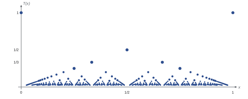
Where are the following continuous? (a) \(D(x) = 1\) if \(x \in \mathbb{Q}\), \(0\) otherwise. (b) \(T(x) = \frac{1}{q}\) if \(x = \frac{p}{q}\) in lowest terms with \(q > 0\), and \(T(x) = 0\) if \(x\) is irrational.
Show solution
- (a) Every interval contains rationals and irrationals, so near any \(c\) the function takes both values 0 and 1. With \(\varepsilon = \frac{1}{2}\) no \(\delta\) works. \(D\), studied by Dirichlet in 1829, is discontinuous everywhere.
- (b) At a rational \(c = \frac{p}{q}\), \(T(c) = \frac{1}{q} > 0\), but irrationals \(x_n \to c\) give \(T(x_n) = 0\). So \(T\) is discontinuous at every rational.
- At an irrational \(c\), let \(\varepsilon > 0\) and choose \(m\) with \(\frac{1}{m} < \varepsilon\). In \((c - 1, c + 1)\) only finitely many rationals have denominator at most \(m\). Choose \(\delta\) smaller than the distance from \(c\) to each of them. Then every \(x\) with \(|x - c| < \delta\) has \(|T(x) - T(c)| = T(x) < \frac{1}{m} < \varepsilon\).
Answer: Dirichlet's function is continuous nowhere. Thomae's function is continuous exactly at the irrationals. These examples show how far real functions can stray from the pen-on-paper picture.
The intermediate value theorem
Theorem (intermediate value theorem). Let \(f: [a, b] \to \mathbb{R}\) be continuous and let \(y\) lie between \(f(a)\) and \(f(b)\). Then there is \(c \in [a, b]\) with \(f(c) = y\).
Proof. Replacing \(f\) by \(f - y\), and if necessary by \(y - f\), we may assume \(f(a) < 0 < f(b)\) and look for \(c\) with \(f(c) = 0\). Let \(S = \{x \in [a, b] : f(x) < 0\}\). It contains \(a\) and is bounded above by \(b\), so \(c = \sup S\) exists, with \(a \le c \le b\). We show \(f(c) = 0\) by ruling out both alternatives.
If \(f(c) < 0\), then \(c < b\), and by continuity with \(\varepsilon = -f(c)\) there is \(\delta > 0\) with \(f(x) < 0\) for \(|x - c| < \delta\). Then some point \(x\) with \(c < x < \min(c + \delta, b)\) lies in \(S\), contradicting that \(c\) is an upper bound.
If \(f(c) > 0\), then \(c > a\), and there is \(\delta > 0\) with \(f(x) > 0\) for \(|x - c| < \delta\). No point of \((c - \delta, c]\) lies in \(S\), so \(c - \delta\) is an upper bound of \(S\), contradicting that \(c\) is the least upper bound. Hence \(f(c) = 0\). \(\blacksquare\)
Each case used continuity to find an interval where \(f\) keeps its sign, and completeness to produce the candidate \(c\). Both are essential. Over \(\mathbb{Q}\) the continuous function \(x^2 - 2\) is negative at 0 and positive at 2 but never zero. And the discontinuous sign function goes from \(-1\) to \(1\) without taking the value \(\frac{1}{2}\).
Bisection: a constructive proof
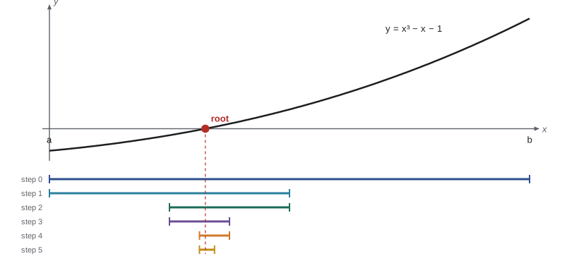
A second proof follows the nested interval idea of lesson 3 and gives an algorithm. Start with \([a_0, b_0] = [a, b]\) where \(f(a) < 0 < f(b)\). At each step evaluate \(f\) at the midpoint \(m\). If \(f(m) = 0\), stop. If \(f(m) < 0\), keep \([m, b_n]\); otherwise keep \([a_n, m]\). The intervals are nested with lengths \(\frac{b - a}{2^n}\), so by the nested interval property they shrink to a single point \(c\), and \(a_n \to c\), \(b_n \to c\). Since \(f(a_n) < 0\) for every \(n\), sequential continuity gives \(f(c) \le 0\); since \(f(b_n) > 0\), it gives \(f(c) \ge 0\). So \(f(c) = 0\).
from fractions import Fraction as F

def bisect(f, a, b, steps):
    """Bisection with exact rational arithmetic; requires f(a) < 0 < f(b)."""
    assert f(a) < 0 < f(b)
    for n in range(1, steps + 1):
        m = (a + b) / 2
        if f(m) == 0:
            return m, m
        if f(m) < 0:
            a = m
        else:
            b = m
        if n in (1, 2, 3, 10, 20, 40):
            print(f"step {n:2}: root in [{float(a):.15f}, {float(b):.15f}], width {float(b - a):.2e}")
    return a, b

cubic = lambda x: x**3 - x - 1          # the real root of x^3 = x + 1
a, b = bisect(cubic, F(1), F(2), 40)
print("f at the ends:", float(cubic(a)), float(cubic(b)))step 1: root in [1.000000000000000, 1.500000000000000], width 5.00e-01 step 2: root in [1.250000000000000, 1.500000000000000], width 2.50e-01 step 3: root in [1.250000000000000, 1.375000000000000], width 1.25e-01 step 10: root in [1.324218750000000, 1.325195312500000], width 9.77e-04 step 20: root in [1.324717521667480, 1.324718475341797], width 9.54e-07 step 40: root in [1.324717957244502, 1.324717957245412], width 9.09e-13 f at the ends: -1.0405479198079439e-12 2.8381131975536757e-12
The root found is the plastic number, about 1.3247. Bisection is slow compared with Newton's method, gaining one binary digit per step, but it is guaranteed to work for every continuous function with a sign change, and the error after \(n\) steps is known in advance: \(\frac{b - a}{2^n}\).
Consequences of the intermediate value theorem
Corollary. Every polynomial of odd degree has a real root. Proof: for \(p(x) = x^n + a_{n-1}x^{n-1} + \dots + a_0\) with \(n\) odd, \(\frac{p(x)}{x^n} \to 1\) as \(x \to \pm\infty\), so \(p(x) > 0\) for large positive \(x\) and \(p(x) < 0\) for large negative \(x\). Apply the theorem on a large enough interval. \(\blacksquare\)
Corollary (fixed points). Every continuous \(f: [0, 1] \to [0, 1]\) has a fixed point, a point with \(f(c) = c\). Proof: \(g(x) = f(x) - x\) has \(g(0) \ge 0\) and \(g(1) \le 0\). \(\blacksquare\) This is the one-dimensional case of the Brouwer fixed point theorem.
Corollary. The continuous image of an interval is an interval. If \(f(x_1) < y < f(x_2)\), the theorem applied between \(x_1\) and \(x_2\) gives a point with value \(y\).
The converse of the intermediate value theorem is false: a function with the intermediate value property need not be continuous. The function \(\sin\frac{1}{x}\) with value 0 at 0 takes every value between any two of its values on any interval, yet it is discontinuous at 0. Darboux proved in 1875 that every derivative has the intermediate value property, whether or not it is continuous; lesson 10 returns to this.
Continuous inverses
The intermediate value theorem also explains why inverse functions of continuous functions are continuous, which is how \(\sqrt[n]{x}\), \(\ln x\) and \(\arcsin x\) inherit continuity from \(x^n\), \(e^x\) and \(\sin x\).
Theorem. Let \(I\) be an interval and \(f: I \to \mathbb{R}\) continuous. Then \(f\) is injective if and only if it is strictly monotone. In that case \(J = f(I)\) is an interval and the inverse \(f^{-1}: J \to I\) is continuous and strictly monotone.
Proof sketch. If \(f\) were injective but not monotone, there would be points \(x_1 < x_2 < x_3\) with \(f(x_2)\) not between \(f(x_1)\) and \(f(x_3)\), say \(f(x_2) > \max(f(x_1), f(x_3))\). A value \(y\) slightly below \(f(x_2)\) and above both ends is taken once in \((x_1, x_2)\) and once in \((x_2, x_3)\) by the intermediate value theorem, contradicting injectivity. So \(f\) is strictly monotone, say increasing, and \(J\) is an interval by the corollary above. The inverse \(g = f^{-1}\) is increasing. An increasing function can be discontinuous only by jumping, and a jump of \(g\) at \(y_0\) would leave a gap in its range \(g(J) = I\). Since \(I\) is an interval it has no gaps, so \(g\) is continuous. \(\blacksquare\)
For example, \(x^n\) is continuous and strictly increasing on \([0, \infty)\), with range \([0, \infty)\) by the intermediate value theorem and the fact that \(x^n \to \infty\). So every non-negative number has a unique non-negative \(n\)-th root, and \(\sqrt[n]{x}\) is continuous. This generalizes the existence of \(\sqrt{2}\) proved in lesson 2 by a direct supremum argument.
Continuity and preimages
There is a definition of continuity that avoids \(\varepsilon\) and \(\delta\). Call a set \(U \subseteq \mathbb{R}\) open if every point of \(U\) has an interval around it inside \(U\). Then \(f: \mathbb{R} \to \mathbb{R}\) is continuous if and only if the preimage \(f^{-1}(U) = \{x : f(x) \in U\}\) is open for every open \(U\). This reformulation is the starting point of topology and of the metric space theory in MATH-341, where intervals are replaced by balls.
Common mistakes
MistakeTreating continuity as having a limit at \(c\).
InsteadContinuity requires the limit to exist and to equal \(f(c)\).
MistakeCalling \(\frac{1}{x}\) discontinuous at 0.
Instead0 is not in its domain; \(\frac{1}{x}\) is continuous on \(\mathbb{R} \setminus \{0\}\). It cannot be extended continuously to 0.
MistakeApplying the intermediate value theorem to a function with a jump.
InsteadContinuity on the whole closed interval is required; the sign function is a counterexample.
MistakeForgetting completeness in the proof.
InsteadThe theorem fails over \(\mathbb{Q}\); the supremum \(c = \sup S\) is where completeness enters.
MistakeAssuming the intermediate value property implies continuity.
Instead\(\sin\frac{1}{x}\) with value 0 at 0 has the property but is discontinuous.
Summary and key terms
- \(f\) is continuous at \(c\) when \(|f(x) - f(c)| < \varepsilon\) for \(|x - c| < \delta\); equivalently \(f(x_n) \to f(c)\) whenever \(x_n \to c\).
- Sums, products, quotients and compositions of continuous functions are continuous.
- Discontinuities are removable, jumps or essential; monotone functions have only countably many jumps.
- Dirichlet's function is continuous nowhere; Thomae's function is continuous exactly at the irrationals.
- The intermediate value theorem: a continuous function on \([a, b]\) takes every value between \(f(a)\) and \(f(b)\). It depends on completeness.
- Bisection turns the theorem into an algorithm with a known error bound.
- Continuous at c
- \(\lim_{x \to c} f(x) = f(c)\), or \(c\) is isolated.
- Removable discontinuity
- The limit exists but differs from the value.
- Jump discontinuity
- Both one-sided limits exist and differ.
- Intermediate value property
- Taking every value between any two values.
- Fixed point
- A point with \(f(c) = c\).
Practice problems
Work each problem on paper first, then reveal the answer to check.
Prove from the definition that \(f(x) = 3x^2\) is continuous at \(c = 1\).
Show answer
\(|3x^2 - 3| = 3|x - 1||x + 1| < 9|x - 1|\) when \(|x - 1| < 1\); take \(\delta = \min(1, \frac{\varepsilon}{9})\).
Show that \(x^5 + x - 1 = 0\) has a root in \((0, 1)\).
Show answer
\(p(0) = -1 < 0 < 1 = p(1)\); apply the intermediate value theorem.
Classify the discontinuity of \(f(x) = \frac{x^2 - 1}{x - 1}\), \(f(1) = 0\), at 1.
Show answer
Removable: the limit is 2 but \(f(1) = 0\).
Suppose \(f\) is continuous and \(f(x) = 0\) for every rational \(x\). Prove \(f = 0\).
Show answer
Each real \(x\) is the limit of rationals \(q_n\) by density, so \(f(x) = \lim f(q_n) = 0\).
Prove that a continuous \(f: [a, b] \to \mathbb{R}\) taking only rational values is constant.
Show answer
If \(f(x_1) \ne f(x_2)\), an irrational lies between them, and the intermediate value theorem would make \(f\) take it.
Lesson quiz · 5 questions
Score 60% or more to complete this lesson.
Create a free account to save your progress, take quizzes and earn a certificate.