
MATH-241 · Lesson 7 of 12 · 27 min
Limits of functions
Calculus courses introduce the limit of a function informally: \(f(x)\) approaches \(L\) as \(x\) approaches \(c\). This lesson makes that statement precise with the epsilon–delta definition, which Weierstrass made standard in his Berlin lectures of the 1860s, building on Cauchy and Bolzano. We prove the limit laws, connect function limits to sequence limits, and develop one-sided limits, limits at infinity and the squeeze theorem. Everything in the next five lessons, from continuity to the integral, is built on this definition.
Limit points
We only want to take limits at points that \(x\) can actually approach from within the domain. Let \(A \subseteq \mathbb{R}\). A point \(c\) is a limit point (or accumulation point) of \(A\) if every interval \((c - \delta, c + \delta)\) contains a point of \(A\) other than \(c\). The point \(c\) itself need not belong to \(A\).
For example, every point of \([0, 1]\) is a limit point of \((0, 1)\), and so is no other point. The set \(\mathbb{Z}\) has no limit points. Every real number is a limit point of \(\mathbb{Q}\), by density. A point of \(A\) that is not a limit point of \(A\) is called isolated.
The definition
Definition. Let \(f: A \to \mathbb{R}\) and let \(c\) be a limit point of \(A\). We say \(\lim_{x \to c} f(x) = L\) if for every \(\varepsilon > 0\) there is \(\delta > 0\) such that \(|f(x) - L| < \varepsilon\) for every \(x \in A\) with \(0 < |x - c| < \delta\).
The condition \(0 < |x - c|\) is essential: the limit ignores the value of \(f\) at \(c\), and \(f\) need not even be defined there. This is what allows the derivative, a limit of difference quotients that are undefined at the point itself, to make sense.
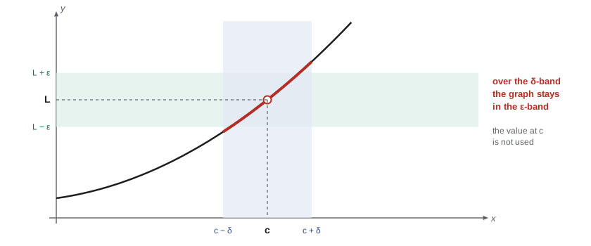
As with sequences, the definition is a game. The opponent picks the tolerance \(\varepsilon\), you answer with \(\delta\), and you win if every admissible \(x\) within \(\delta\) of \(c\) has \(f(x)\) within \(\varepsilon\) of \(L\). The limit is \(L\) if you can win for every \(\varepsilon\).
Worked problem
A quadratic limit
Prove \(\lim_{x \to 2} x^2 = 4\).
Show solution
- Scratch work: \(|x^2 - 4| = |x - 2| \, |x + 2|\). If \(|x - 2| < 1\) then \(1 < x < 3\), so \(|x + 2| < 5\).
- Proof: let \(\varepsilon > 0\) and set \(\delta = \min(1, \frac{\varepsilon}{5})\).
- If \(0 < |x - 2| < \delta\), then \(|x + 2| < 5\) and \(|x^2 - 4| < 5 \cdot \frac{\varepsilon}{5} = \varepsilon\).
Answer: The trick of first restricting \(\delta \le 1\) to bound the extra factor is used constantly.
Worked problem
A limit where f is not defined
Prove \(\lim_{x \to 3} \frac{x^2 - 9}{x - 3} = 6\).
Show solution
- The function is defined on \(\mathbb{R} \setminus \{3\}\), and 3 is a limit point of that set.
- For \(x \ne 3\), \(\frac{x^2 - 9}{x - 3} = x + 3\), so \(\big|\frac{x^2 - 9}{x - 3} - 6\big| = |x - 3|\).
- Given \(\varepsilon\), take \(\delta = \varepsilon\).
Answer: The limit is 6 even though the function has no value at 3. Removing a single point does not affect a limit.
Uniqueness. If \(\lim_{x \to c} f(x) = L\) and \(= M\), then \(L = M\). The proof is the same as for sequences: given \(\varepsilon > 0\), take \(\delta\) small enough for both limits and choose some \(x \in A\) with \(0 < |x - c| < \delta\), which exists because \(c\) is a limit point. Then \(|L - M| \le |L - f(x)| + |f(x) - M| < 2\varepsilon\). This is where the limit point condition is used: at an isolated point every \(L\) would satisfy the definition vacuously.
The sequential criterion
Theorem (sequential criterion). \(\lim_{x \to c} f(x) = L\) if and only if for every sequence \((x_n)\) in \(A\) with \(x_n \ne c\) and \(x_n \to c\), we have \(f(x_n) \to L\).
Proof. Suppose the limit is \(L\), and let \(x_n \to c\) with \(x_n \ne c\). Given \(\varepsilon\), take \(\delta\) from the definition, then \(N\) with \(|x_n - c| < \delta\) for \(n \ge N\). For such \(n\), \(0 < |x_n - c| < \delta\), so \(|f(x_n) - L| < \varepsilon\).
Conversely, suppose the limit is not \(L\). Negating the definition, there is \(\varepsilon_0 > 0\) such that for every \(\delta > 0\) some \(x \in A\) has \(0 < |x - c| < \delta\) but \(|f(x) - L| \ge \varepsilon_0\). Apply this with \(\delta = \frac{1}{n}\) to get \(x_n\). Then \(x_n \to c\), \(x_n \ne c\), but \(f(x_n)\) does not tend to \(L\). \(\blacksquare\)
The criterion transfers everything we proved about sequences. It also gives the standard method for proving a limit does not exist: find two sequences tending to \(c\) along which \(f\) has different limits.
Worked problem
A limit that does not exist
Show that \(\lim_{x \to 0} \sin\frac{1}{x}\) does not exist.
Show solution
- Let \(x_n = \frac{1}{2\pi n}\). Then \(x_n \to 0\) and \(\sin\frac{1}{x_n} = \sin(2\pi n) = 0\).
- Let \(y_n = \frac{1}{2\pi n + \pi/2}\). Then \(y_n \to 0\) and \(\sin\frac{1}{y_n} = 1\).
- If the limit were \(L\), both sequences of values would converge to \(L\), forcing \(0 = L = 1\).
Answer: The function oscillates infinitely often between \(-1\) and \(1\) near 0, so no limit exists. By contrast \(x \sin\frac{1}{x} \to 0\), by the squeeze theorem below.
The limit laws
Theorem. Suppose \(\lim_{x \to c} f(x) = L\) and \(\lim_{x \to c} g(x) = M\). Then
\[\lim_{x \to c} (f + g)(x) = L + M, \qquad \lim_{x \to c} (fg)(x) = LM, \qquad \lim_{x \to c} \frac{f(x)}{g(x)} = \frac{L}{M} \text{ if } M \ne 0.\]
Proof. Take any sequence \(x_n \to c\) with \(x_n \ne c\). Then \(f(x_n) \to L\) and \(g(x_n) \to M\), so by the algebraic limit theorem for sequences (lesson 4) \(f(x_n) + g(x_n) \to L + M\), and similarly for products and quotients. For the quotient, \(g(x) \ne 0\) for \(x\) near \(c\), since \(|g(x)| > \frac{|M|}{2}\) once \(|g(x) - M| < \frac{|M|}{2}\). By the sequential criterion the limits hold. \(\blacksquare\)
With \(\lim_{x \to c} x = c\) and the limit of a constant, the laws give the limit of every polynomial at every point by substitution, and of every rational function wherever its denominator is non-zero.
Theorem (squeeze). If \(g(x) \le f(x) \le h(x)\) for \(x\) near \(c\) and \(\lim g = \lim h = L\), then \(\lim_{x \to c} f(x) = L\). The proof follows from the squeeze theorem for sequences.
Worked problem
The fundamental trigonometric limit
Prove \(\lim_{x \to 0} \frac{\sin x}{x} = 1\), assuming the inequality \(\cos x \le \frac{\sin x}{x} \le 1\) for \(0 < |x| < \frac{\pi}{2}\).
Show solution
- The inequality comes from comparing the areas of two triangles and a circular sector in the unit circle: \(\frac{1}{2}\sin x \cos x \le \frac{1}{2}x \le \frac{1}{2}\tan x\) for \(0 < x < \frac{\pi}{2}\), then dividing by \(\frac{1}{2}\sin x\) and taking reciprocals.
- Both sides are even in \(x\), so the inequality holds for negative \(x\) too.
- Since \(\cos x \to 1\) as \(x \to 0\), the squeeze theorem gives the limit 1.
Answer: This limit is the key to differentiating \(\sin\). A fully rigorous treatment defines \(\sin\) by its power series, which MATH-341 develops.
One-sided limits and limits involving infinity
The right-hand limit \(\lim_{x \to c^+} f(x) = L\) means the definition holds for \(x\) with \(c < x < c + \delta\). The left-hand limit uses \(c - \delta < x < c\). When \(c\) is a limit point from both sides, \(\lim_{x \to c} f(x) = L\) if and only if both one-sided limits exist and equal \(L\).
For example, the sign function \(\operatorname{sgn}(x)\), equal to \(-1\), \(0\) or \(1\) according as \(x < 0\), \(x = 0\) or \(x > 0\), has right-hand limit 1 and left-hand limit \(-1\) at 0, so it has no two-sided limit there.
Limits at infinity. \(\lim_{x \to \infty} f(x) = L\) means: for every \(\varepsilon > 0\) there is \(M\) with \(|f(x) - L| < \varepsilon\) for all \(x > M\) in the domain. This is the function analogue of a sequence limit; for instance \(\frac{1}{x} \to 0\) by the Archimedean property.
Infinite limits. \(\lim_{x \to c} f(x) = \infty\) means: for every \(M\) there is \(\delta > 0\) with \(f(x) > M\) whenever \(0 < |x - c| < \delta\). For instance \(\frac{1}{x^2} \to \infty\) as \(x \to 0\): given \(M > 0\), take \(\delta = \frac{1}{\sqrt{M}}\). Infinite limits do not exist as real numbers; the notation records a specific way of failing to converge.
| Statement | Tolerance on output | Closeness of input |
|---|---|---|
| \(\lim_{x \to c} f(x) = L\) | \(|f(x) - L| < \varepsilon\) | \(0 < |x - c| < \delta\) |
| \(\lim_{x \to c^+} f(x) = L\) | \(|f(x) - L| < \varepsilon\) | \(c < x < c + \delta\) |
| \(\lim_{x \to \infty} f(x) = L\) | \(|f(x) - L| < \varepsilon\) | \(x > M\) |
| \(\lim_{x \to c} f(x) = \infty\) | \(f(x) > M\) | \(0 < |x - c| < \delta\) |
| \(\lim_{n \to \infty} a_n = L\) | \(|a_n - L| < \varepsilon\) | \(n \ge N\) |
Composition of limits
If \(\lim_{x \to c} g(x) = b\) and \(\lim_{y \to b} f(y) = L\), is \(\lim_{x \to c} f(g(x)) = L\)? Not always. Let \(g(x) = 0\) for all \(x\), and let \(f(y) = 1\) for \(y \ne 0\) and \(f(0) = 0\). Then \(\lim_{y \to 0} f(y) = 1\) but \(f(g(x)) = 0\) for every \(x\). The trouble is that \(g(x)\) hits \(b\) itself, where the limit of \(f\) says nothing. The composition rule is valid if either \(g(x) \ne b\) for \(x\) near \(c\), or \(f\) is continuous at \(b\), which is the topic of the next lesson.
Computing a delta
For many functions the best \(\delta\) can be found numerically by shrinking it until the condition holds on a fine grid. This does not prove anything, since a grid checks only finitely many points, but it shows how \(\delta\) must shrink as \(\varepsilon\) does, and it is a useful way to check a hand computation.
from fractions import Fraction as F

def works(f, c, L, eps, delta, samples=4000):
    """Check |f(x) - L| < eps at grid points with 0 < |x - c| < delta."""
    for i in range(1, samples + 1):
        h = delta * F(i, samples + 1)
        for x in (c - h, c + h):
            if abs(f(x) - L) >= eps:
                return False
    return True

def find_delta(f, c, L, eps):
    delta = F(1)
    while not works(f, c, L, eps, delta, samples=200):
        delta /= 2
    return delta

square = lambda x: x * x
for eps in (F(1), F(1, 10), F(1, 100), F(1, 1000)):
    d = find_delta(square, F(2), F(4), eps)
    proof_delta = min(F(1), eps / 5)
    best = (4 + float(eps)) ** 0.5 - 2           # largest delta that works
    print(f"eps = {float(eps):<6} halving: {float(d):.6f}  proof: {float(proof_delta):.6f}  "
f"largest: {best:.6f} proof delta passes: {works(square, F(2), F(4), eps, proof_delta)}")eps = 1.0 halving: 0.125000 proof: 0.200000 largest: 0.236068 proof delta passes: True eps = 0.1 halving: 0.015625 proof: 0.020000 largest: 0.024846 proof delta passes: True eps = 0.01 halving: 0.001953 proof: 0.002000 largest: 0.002498 proof delta passes: True eps = 0.001 halving: 0.000244 proof: 0.000200 largest: 0.000250 proof delta passes: True
The halving search can only return a power of 2. The largest \(\delta\) that works is \(\sqrt{4 + \varepsilon} - 2\), since \(x^2 - 4\) grows faster to the right of 2 than it falls to the left. The proof's \(\delta = \min(1, \frac{\varepsilon}{5})\) is a little smaller than that, which is fine: the definition asks only that some \(\delta\) works. A proof needs a \(\delta\) that is easy to justify, not the largest possible one.
From intuition to definition
Eighteenth-century analysts such as Euler worked confidently with limits without defining them, and their results were usually right. The trouble appeared at the edges: infinite series of functions whose sums jumped, and arguments that divided by quantities that were later set to zero, which Berkeley had mocked in The Analyst of 1734 as the ghosts of departed quantities. Cauchy's 1821 definition still spoke of variables approaching values. The fully static version, with \(\varepsilon\) and \(\delta\) as fixed numbers and no motion at all, is due to Weierstrass and his students, and it removes every appeal to time or motion. The phrase \(x\) approaches \(c\) survives as a figure of speech, but the definition is a statement about all \(x\) in a set, quantified in a definite order.
That order matters. The definition reads: for every \(\varepsilon\) there exists \(\delta\) such that for every \(x\). Swapping the first two quantifiers, there exists \(\delta\) such that for every \(\varepsilon\), would force \(f(x) = L\) for every \(x\) near \(c\), a far stronger and rarely useful condition. Reading quantifiers in order, and writing proofs that choose \(\delta\) only after \(\varepsilon\) is given, is the main skill this lesson trains.
Common mistakes
MistakeLetting \(\delta\) depend on \(x\).
Instead\(\delta\) may depend on \(\varepsilon\) and \(c\), but must work for every \(x\) in the punctured interval at once.
MistakeEvaluating \(f(c)\) to find the limit.
InsteadThe limit ignores \(f(c)\); it equals \(f(c)\) only when \(f\) is continuous at \(c\).
MistakeConcluding a limit exists because it exists along one sequence.
InsteadThe sequential criterion requires every sequence \(x_n \to c\) with \(x_n \ne c\).
MistakeWriting \(\lim f(x) = \infty\) and treating \(\infty\) as a number in later algebra.
InsteadAn infinite limit means the limit does not exist in \(\mathbb{R}\); laws like \(L + M\) do not apply.
MistakeComposing limits without checking.
Instead\(f(g(x))\) need not tend to \(\lim f\) unless \(g(x) \ne b\) nearby or \(f\) is continuous at \(b\).
Summary and key terms
- \(\lim_{x \to c} f(x) = L\): for every \(\varepsilon > 0\) there is \(\delta > 0\) with \(|f(x) - L| < \varepsilon\) whenever \(0 < |x - c| < \delta\).
- Limits are taken at limit points of the domain and ignore the value at \(c\).
- The sequential criterion turns function limits into sequence limits, proving the limit laws and squeeze theorem.
- Two sequences with different limiting values prove a limit does not exist.
- One-sided limits, limits at infinity and infinite limits share the same tolerance-and-neighbourhood structure.
- Limit point
- A point \(c\) such that every neighbourhood contains points of \(A\) other than \(c\).
- Epsilon–delta limit
- \(|f(x) - L| < \varepsilon\) whenever \(0 < |x - c| < \delta\).
- Sequential criterion
- \(f(x) \to L\) iff \(f(x_n) \to L\) for all \(x_n \to c\), \(x_n \ne c\).
- One-sided limit
- A limit using only \(x > c\) or only \(x < c\).
- Infinite limit
- \(f(x)\) eventually exceeds every bound as \(x \to c\).
Practice problems
Work each problem on paper first, then reveal the answer to check.
Prove \(\lim_{x \to 1} (3x + 2) = 5\).
Show answer
\(|3x + 2 - 5| = 3|x - 1|\); take \(\delta = \frac{\varepsilon}{3}\).
Prove \(\lim_{x \to 4} \sqrt{x} = 2\).
Show answer
\(|\sqrt{x} - 2| = \frac{|x - 4|}{\sqrt{x} + 2} \le \frac{|x - 4|}{2}\); take \(\delta = \min(4, 2\varepsilon)\).
Prove \(\lim_{x \to 0} x \sin\frac{1}{x} = 0\).
Show answer
\(|x \sin\frac{1}{x}| \le |x|\); take \(\delta = \varepsilon\), or use the squeeze theorem.
Show that \(\lim_{x \to 0} \frac{|x|}{x}\) does not exist.
Show answer
Along \(x_n = \frac{1}{n}\) the value is 1; along \(-\frac{1}{n}\) it is \(-1\).
Let \(f(x) = 1\) for rational \(x\) and \(0\) for irrational \(x\). At which \(c\) does \(\lim_{x \to c} f(x)\) exist?
Show answer
None: by density, rational and irrational sequences tend to every \(c\), giving limits 1 and 0.
Lesson quiz · 5 questions
Score 60% or more to complete this lesson.
Create a free account to save your progress, take quizzes and earn a certificate.