
MATH-221 · Lesson 9 of 12 · 23 min
Inner product spaces and orthogonality
So far our vector spaces have had no notion of length or angle. Linear independence, dimension, eigenvalues and Jordan forms are all purely algebraic. Geometry enters with an inner product, a rule for multiplying two vectors to get a scalar that generalizes the dot product. Once a space has an inner product we can measure lengths, distances and angles, talk about perpendicular vectors, and project onto subspaces. Remarkably, the same few axioms cover the dot product on \(\mathbb{R}^n\), integrals of products of functions, and the trace of products of matrices, so a single theory handles least squares fitting, Fourier series and the geometry of data. This lesson sets up that theory and proves its two foundational results, the Cauchy–Schwarz inequality and the Gram–Schmidt process.
The axioms
An inner product on a real vector space \(V\) is a function \(\langle \cdot, \cdot \rangle : V \times V \to \mathbb{R}\) such that for all vectors \(\mathbf{u}, \mathbf{v}, \mathbf{w}\) and scalars \(c\):
- linearity in the first slot: \(\langle \mathbf{u} + \mathbf{w}, \mathbf{v} \rangle = \langle \mathbf{u}, \mathbf{v} \rangle + \langle \mathbf{w}, \mathbf{v} \rangle\) and \(\langle c\mathbf{u}, \mathbf{v} \rangle = c\langle \mathbf{u}, \mathbf{v} \rangle\);
- symmetry: \(\langle \mathbf{u}, \mathbf{v} \rangle = \langle \mathbf{v}, \mathbf{u} \rangle\);
- positivity: \(\langle \mathbf{v}, \mathbf{v} \rangle > 0\) for every \(\mathbf{v} \ne \mathbf{0}\).
Symmetry plus linearity in the first slot give linearity in the second. Over \(\mathbb{C}\), symmetry is replaced by conjugate symmetry, \(\langle \mathbf{u}, \mathbf{v} \rangle = \overline{\langle \mathbf{v}, \mathbf{u} \rangle}\), which makes \(\langle \mathbf{v}, \mathbf{v} \rangle\) real and the second slot conjugate-linear. The standard complex inner product is \(\langle \mathbf{u}, \mathbf{v} \rangle = \sum u_i\overline{v_i}\); without the conjugate, the vector \((1, i)\) would have length zero. A vector space with an inner product is an inner product space. The norm is \(\|\mathbf{v}\| = \sqrt{\langle \mathbf{v}, \mathbf{v} \rangle}\) and the distance between vectors is \(\|\mathbf{u} - \mathbf{v}\|\).
| Space | Inner product | Comment |
|---|---|---|
| \(\mathbb{R}^n\) | \(\mathbf{u} \cdot \mathbf{v} = \sum u_iv_i\) | The dot product from MATH-125 |
| \(\mathbb{R}^n\) | \(\mathbf{u}^{T}W\mathbf{v}\) with \(W\) symmetric positive definite | Weighted inner products, used in weighted least squares |
| \(C[a, b]\) | \(\int_a^b f(t)g(t)\,dt\) | Basis of Fourier series and function approximation |
| \(P_n\) | \(\sum_{i=0}^{n} p(t_i)q(t_i)\) at \(n + 1\) distinct nodes | Discrete inner product for data fitting |
| \(M_{m \times n}\) | \(\operatorname{tr}(A^{T}B) = \sum a_{ij}b_{ij}\) | The Frobenius inner product |
| \(\mathbb{C}^n\) | \(\sum u_i\overline{v_i}\) | Conjugate needed for positivity |
Positivity is the axiom that can fail. On \(P_2\), \(\langle p, q \rangle = p(0)q(0) + p(1)q(1)\) is linear and symmetric but not positive: the nonzero polynomial \(t(t - 1)\) has \(\langle p, p \rangle = 0\). With three distinct nodes it becomes an inner product, because a nonzero quadratic cannot vanish at three points. Every inner product on \(\mathbb{R}^n\) has the form \(\mathbf{u}^{T}W\mathbf{v}\) for some symmetric positive definite \(W\), namely the Gram matrix with entries \(W_{ij} = \langle \mathbf{e}_i, \mathbf{e}_j \rangle\). Lesson 11 explains how to recognize positive definite matrices.
Cauchy–Schwarz and the triangle inequality
Theorem (Cauchy–Schwarz). For all \(\mathbf{u}, \mathbf{v}\) in an inner product space, \(|\langle \mathbf{u}, \mathbf{v} \rangle| \le \|\mathbf{u}\|\,\|\mathbf{v}\|\), with equality exactly when one is a multiple of the other.
Proof (real case). If \(\mathbf{v} = \mathbf{0}\) both sides are 0. Otherwise, for every real \(t\), positivity gives
This quadratic in \(t\) is never negative, so its discriminant is not positive: \(4\langle \mathbf{u}, \mathbf{v} \rangle^2 - 4\|\mathbf{u}\|^2\|\mathbf{v}\|^2 \le 0\). Equality means the quadratic has a root \(t\), so \(\mathbf{u} = t\mathbf{v}\). A slicker route, which works over \(\mathbb{C}\) too, takes \(t = \langle \mathbf{u}, \mathbf{v} \rangle/\|\mathbf{v}\|^2\), the value that minimizes the quadratic; this choice reappears below as the projection coefficient.
Cauchy–Schwarz lets us define the angle between nonzero real vectors by \(\cos\theta = \langle \mathbf{u}, \mathbf{v} \rangle/(\|\mathbf{u}\|\|\mathbf{v}\|)\), since the ratio lies in \([-1, 1]\). In statistics, the correlation coefficient of two centred data vectors is exactly this cosine, which is why it lies between \(-1\) and 1. Applied to the integral inner product it gives \(\big(\int fg\big)^2 \le \int f^2 \int g^2\), an inequality used constantly in analysis.
Corollary (triangle inequality). \(\|\mathbf{u} + \mathbf{v}\| \le \|\mathbf{u}\| + \|\mathbf{v}\|\). Proof: \(\|\mathbf{u} + \mathbf{v}\|^2 = \|\mathbf{u}\|^2 + 2\langle \mathbf{u}, \mathbf{v} \rangle + \|\mathbf{v}\|^2 \le \|\mathbf{u}\|^2 + 2\|\mathbf{u}\|\|\mathbf{v}\| + \|\mathbf{v}\|^2 = (\|\mathbf{u}\| + \|\mathbf{v}\|)^2\). Another identity worth knowing is the parallelogram law, \(\|\mathbf{u} + \mathbf{v}\|^2 + \|\mathbf{u} - \mathbf{v}\|^2 = 2\|\mathbf{u}\|^2 + 2\|\mathbf{v}\|^2\), which characterizes the norms that come from inner products. The taxicab norm \(|x| + |y|\) on \(\mathbb{R}^2\) fails it, so it comes from no inner product.
Orthogonality and orthonormal bases
Vectors are orthogonal if \(\langle \mathbf{u}, \mathbf{v} \rangle = 0\). For orthogonal vectors the Pythagorean theorem \(\|\mathbf{u} + \mathbf{v}\|^2 = \|\mathbf{u}\|^2 + \|\mathbf{v}\|^2\) holds in any inner product space, with the same one-line proof. A list is orthonormal if its vectors are pairwise orthogonal and each has norm 1.
Theorem. An orthonormal list is linearly independent, and if \(\mathbf{e}_1, \dots, \mathbf{e}_n\) is an orthonormal basis then every vector satisfies
Proof: take the inner product of \(\sum c_j\mathbf{e}_j = \mathbf{v}\) with \(\mathbf{e}_k\); orthonormality kills every term except \(c_k\). With \(\mathbf{v} = \mathbf{0}\) this gives independence. The second identity is Parseval's identity. The point is that coordinates in an orthonormal basis cost one inner product each, with no linear system to solve. Compare lesson 2, where finding coordinates meant row reduction.
The Gram–Schmidt process
Theorem. Every finite-dimensional inner product space has an orthonormal basis. More precisely, if \(\mathbf{v}_1, \dots, \mathbf{v}_n\) is linearly independent, define
Then \(\mathbf{e}_1, \dots, \mathbf{e}_n\) is orthonormal and \(\operatorname{span}(\mathbf{e}_1, \dots, \mathbf{e}_k) = \operatorname{span}(\mathbf{v}_1, \dots, \mathbf{v}_k)\) for every \(k\).
Proof by induction on \(k\). Suppose \(\mathbf{e}_1, \dots, \mathbf{e}_{k-1}\) are orthonormal with the same span as \(\mathbf{v}_1, \dots, \mathbf{v}_{k-1}\). Then \(\mathbf{w}_k \ne \mathbf{0}\), since otherwise \(\mathbf{v}_k\) would lie in the span of the earlier \(\mathbf{v}_j\), contradicting independence. For \(i < k\), \(\langle \mathbf{w}_k, \mathbf{e}_i \rangle = \langle \mathbf{v}_k, \mathbf{e}_i \rangle - \langle \mathbf{v}_k, \mathbf{e}_i \rangle = 0\), so \(\mathbf{e}_k\) is a unit vector orthogonal to the earlier ones. The spans agree because \(\mathbf{e}_k\) is a combination of \(\mathbf{v}_k\) and \(\mathbf{e}_1, \dots, \mathbf{e}_{k-1}\), and conversely \(\mathbf{v}_k\) is a combination of \(\mathbf{e}_1, \dots, \mathbf{e}_k\).
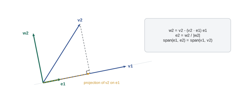
Corollary. Any orthonormal list extends to an orthonormal basis: extend it to a basis, then apply Gram–Schmidt, which leaves the original orthonormal vectors unchanged. And by Gram–Schmidt applied to a triangularizing basis, Schur's theorem from lesson 7 follows: every complex matrix is unitarily similar to an upper triangular one.
Worked problem
Orthogonal polynomials
Apply Gram–Schmidt to \(1, t, t^2\) in \(P_2\) with \(\langle p, q \rangle = \int_{-1}^{1} p(t)q(t)\,dt\), without normalizing.
Show solution
- \(\mathbf{w}_1 = 1\), with \(\langle 1, 1 \rangle = 2\).
- \(\langle t, 1 \rangle = \int_{-1}^{1} t\,dt = 0\), so \(\mathbf{w}_2 = t\), with \(\langle t, t \rangle = 2/3\).
- \(\langle t^2, 1 \rangle = 2/3\) and \(\langle t^2, t \rangle = 0\), so \(\mathbf{w}_3 = t^2 - \frac{2/3}{2}\cdot 1 = t^2 - \frac13\).
- Check: \(\int_{-1}^{1}(t^2 - \frac13)\,dt = \frac23 - \frac23 = 0\).
Answer: \(1, t, t^2 - \frac13\). Scaled so that each equals 1 at \(t = 1\), these are the Legendre polynomials \(1, t, \frac12(3t^2 - 1)\), used in Gaussian quadrature and in solving physical problems with spherical symmetry.
Orthogonal complements
For a subset \(U\) of \(V\), the orthogonal complement is \(U^{\perp} = \{\mathbf{v} : \langle \mathbf{v}, \mathbf{u} \rangle = 0 \text{ for all } \mathbf{u} \in U\}\). It is always a subspace. In \(\mathbb{R}^3\), the complement of a line through the origin is the perpendicular plane. In MATH-125 you met the matrix version: the null space of \(A\) is the orthogonal complement of its row space.
Theorem. If \(U\) is a finite-dimensional subspace of \(V\), then \(V = U \oplus U^{\perp}\), and if \(V\) is finite-dimensional, \(\dim U^{\perp} = \dim V - \dim U\) and \((U^{\perp})^{\perp} = U\). Proof: pick an orthonormal basis \(\mathbf{e}_1, \dots, \mathbf{e}_m\) of \(U\). For any \(\mathbf{v}\), write \(\mathbf{v} = \mathbf{u} + (\mathbf{v} - \mathbf{u})\) with \(\mathbf{u} = \sum\langle \mathbf{v}, \mathbf{e}_j \rangle\mathbf{e}_j\); the second piece is orthogonal to each \(\mathbf{e}_j\) and so lies in \(U^{\perp}\). The intersection \(U \cap U^{\perp}\) is zero because a vector orthogonal to itself is zero. The vector \(\mathbf{u}\) is the orthogonal projection of \(\mathbf{v}\) onto \(U\), the main subject of lesson 10.
Linear functionals and adjoints
In a finite-dimensional inner product space, every linear functional \(\varphi : V \to \mathbb{F}\) has the form \(\varphi(\mathbf{v}) = \langle \mathbf{v}, \mathbf{u} \rangle\) for exactly one vector \(\mathbf{u}\). This is the Riesz representation theorem; with an orthonormal basis, \(\mathbf{u} = \sum\overline{\varphi(\mathbf{e}_j)}\mathbf{e}_j\). For example, on \(P_2\) with the integral inner product, evaluation at \(t = 0\) is represented by a specific quadratic.
Using Riesz, every operator \(T\) on \(V\) has an adjoint \(T^{*}\) defined by \(\langle T\mathbf{u}, \mathbf{v} \rangle = \langle \mathbf{u}, T^{*}\mathbf{v} \rangle\) for all \(\mathbf{u}, \mathbf{v}\). In an orthonormal basis, the matrix of \(T^{*}\) is the conjugate transpose of the matrix of \(T\); in a non-orthonormal basis it is not. Operators with \(T^{*} = T\) are self-adjoint, and they are the subject of the spectral theorem in lesson 11. The fundamental identities \(\ker T^{*} = (\operatorname{im}T)^{\perp}\) and \(\operatorname{im}T^{*} = (\ker T)^{\perp}\) generalize the four fundamental subspaces of a matrix.
Gram–Schmidt in floating point
The formula above is classical Gram–Schmidt: each \(\mathbf{w}_k\) is computed from the original \(\mathbf{v}_k\). Modified Gram–Schmidt instead subtracts the components one at a time from the running vector, which is the same in exact arithmetic but much more accurate in floating point when the input vectors are nearly dependent. The code measures the loss of orthogonality, \(\|Q^{T}Q - I\|\), for both versions on columns of a Hilbert matrix, a standard ill-conditioned test case.
import numpy as np

def classical_gs(V):
    Q = np.zeros_like(V)
    for k in range(V.shape[1]):
        w = V[:, k] - Q[:, :k] @ (Q[:, :k].T @ V[:, k])
        Q[:, k] = w / np.linalg.norm(w)
    return Q

def modified_gs(V):
    Q = V.copy()
    for k in range(V.shape[1]):
        Q[:, k] /= np.linalg.norm(Q[:, k])
        for j in range(k + 1, V.shape[1]):
            Q[:, j] -= (Q[:, k] @ Q[:, j]) * Q[:, k]
    return Q

for n in (4, 8, 12):
    H = np.array([[1.0 / (i + j + 1) for j in range(n)] for i in range(n)])
    cond = np.linalg.cond(H)
    for name, f in (("classical", classical_gs), ("modified ", modified_gs)):
        Q = f(H)
        loss = np.linalg.norm(Q.T @ Q - np.eye(n))
        print(f"n={n:2d}  cond={cond:.1e}  {name}: loss of orthogonality {loss:.1e}")
    Qh, _ = np.linalg.qr(H)
print(f"n={n:2d} Householder QR (numpy): loss {np.linalg.norm(Qh.T @ Qh - np.eye(n)):.1e}")n= 4 cond=1.6e+04 classical: loss of orthogonality 2.7e-11 n= 4 cond=1.6e+04 modified : loss of orthogonality 4.2e-13 n= 4 Householder QR (numpy): loss 7.9e-16 n= 8 cond=1.5e+10 classical: loss of orthogonality 1.4e+00 n= 8 cond=1.5e+10 modified : loss of orthogonality 3.6e-07 n= 8 Householder QR (numpy): loss 7.3e-16 n=12 cond=1.6e+16 classical: loss of orthogonality 5.5e+00 n=12 cond=1.6e+16 modified : loss of orthogonality 1.6e-01 n=12 Householder QR (numpy): loss 1.7e-15
As the condition number grows, classical Gram–Schmidt produces vectors that are far from orthogonal, while modified Gram–Schmidt loses orthogonality roughly in proportion to the condition number, and Householder QR, which numpy uses, stays orthogonal to machine precision. Lesson 10 explains the QR factorization these algorithms produce and why it is the right way to solve least squares problems.
Common mistakes
MistakeForgetting the complex conjugate in the complex inner product.
InsteadUse \(\sum u_i\overline{v_i}\); otherwise vectors such as \((1, i)\) have zero length.
MistakeAssuming every symmetric bilinear form is an inner product.
InsteadPositivity must be checked; \(p(0)q(0) + p(1)q(1)\) fails on \(P_2\).
MistakeComputing coordinates in an orthogonal (not orthonormal) basis as \(\langle \mathbf{v}, \mathbf{w}_j \rangle\).
InsteadDivide by \(\|\mathbf{w}_j\|^2\): the coefficient is \(\langle \mathbf{v}, \mathbf{w}_j \rangle/\langle \mathbf{w}_j, \mathbf{w}_j \rangle\).
MistakeTaking the matrix of the adjoint to be the transpose in any basis.
InsteadThat holds in an orthonormal basis; otherwise the Gram matrix enters.
MistakeUsing classical Gram–Schmidt for nearly dependent vectors.
InsteadUse modified Gram–Schmidt or Householder QR.
Summary and key terms
- An inner product is linear, symmetric (conjugate symmetric over \(\mathbb{C}\)) and positive; it defines norms, distances and angles.
- Cauchy–Schwarz and the triangle inequality hold in every inner product space.
- Coordinates in an orthonormal basis are inner products, and Parseval gives the norm.
- Gram–Schmidt turns any basis into an orthonormal one with the same nested spans.
- \(V = U \oplus U^{\perp}\) for finite-dimensional \(U\).
- Every functional is an inner product with a fixed vector, and every operator has an adjoint.
- In floating point, modified Gram–Schmidt or Householder QR should replace the classical formula.
- inner product
- A positive, symmetric (or conjugate symmetric) form linear in its first slot.
- norm
- \(\|\mathbf{v}\| = \sqrt{\langle \mathbf{v}, \mathbf{v} \rangle}\).
- Cauchy–Schwarz inequality
- \(|\langle \mathbf{u}, \mathbf{v} \rangle| \le \|\mathbf{u}\|\|\mathbf{v}\|\).
- orthonormal basis
- A basis of pairwise orthogonal unit vectors.
- Gram–Schmidt process
- An algorithm that orthonormalizes a list while preserving nested spans.
- orthogonal complement
- The set of vectors orthogonal to every vector of a subset.
- adjoint
- The operator with \(\langle T\mathbf{u}, \mathbf{v} \rangle = \langle \mathbf{u}, T^{*}\mathbf{v} \rangle\).
- Gram matrix
- The matrix of inner products \(\langle \mathbf{b}_i, \mathbf{b}_j \rangle\) of a basis.
Practice problems
Work each problem on paper first, then reveal the answer to check.
Show that \(\langle A, B \rangle = \operatorname{tr}(A^{T}B)\) is an inner product on \(M_{2 \times 2}\).
Show answer
It equals \(\sum a_{ij}b_{ij}\), the dot product of the flattened matrices.
Prove the parallelogram law.
Show answer
Expand \(\|\mathbf{u} \pm \mathbf{v}\|^2\) and add; the cross terms cancel.
Prove that \(\big(\sum_{i=1}^{n} a_i\big)^2 \le n\sum a_i^2\).
Show answer
Apply Cauchy–Schwarz to \((a_1, \dots, a_n)\) and \((1, \dots, 1)\).
Orthonormalize \((1, 1, 0)\), \((1, 0, 1)\) in \(\mathbb{R}^3\).
Show answer
\(\mathbf{e}_1 = \frac{1}{\sqrt2}(1, 1, 0)\); \(\mathbf{w}_2 = (1, 0, 1) - \frac12(1, 1, 0) = (\frac12, -\frac12, 1)\); \(\mathbf{e}_2 = \frac{1}{\sqrt6}(1, -1, 2)\).
Prove that \(U^{\perp}\) is a subspace for any subset \(U\).
Show answer
It contains 0, and if \(\langle \mathbf{v}, \mathbf{u} \rangle = \langle \mathbf{w}, \mathbf{u} \rangle = 0\) then \(\langle a\mathbf{v} + b\mathbf{w}, \mathbf{u} \rangle = 0\).
Prove that \(\ker T^{*} = (\operatorname{im} T)^{\perp}\).
Show answer
\(T^{*}\mathbf{v} = 0\) iff \(\langle \mathbf{u}, T^{*}\mathbf{v} \rangle = 0\) for all \(\mathbf{u}\) iff \(\langle T\mathbf{u}, \mathbf{v} \rangle = 0\) for all \(\mathbf{u}\).
Lesson quiz · 5 questions
Score 60% or more to complete this lesson.
Create a free account to save your progress, take quizzes and earn a certificate.