
MATH-221 · Lesson 11 of 12 · 22 min
The spectral theorem and quadratic forms
Lessons 6 to 8 showed that diagonalization can fail and that, even when it succeeds, the eigenvector basis may be badly skewed. For one large and important class of operators neither problem arises. A self-adjoint operator on a real inner product space, which in an orthonormal basis means a symmetric matrix, always has real eigenvalues and an orthonormal basis of eigenvectors. This is the spectral theorem, and it is arguably the most used theorem in applied linear algebra. Covariance matrices, Hessians, stiffness matrices, graph Laplacians and the matrices \(A^{T}A\) of least squares are all symmetric. This lesson proves the theorem, extends it to normal operators over \(\mathbb{C}\), and applies it to quadratic forms: classifying them, finding their principal axes and optimizing them on the unit sphere.
Self-adjoint operators
Recall from lesson 9 that the adjoint \(T^{*}\) satisfies \(\langle T\mathbf{u}, \mathbf{v} \rangle = \langle \mathbf{u}, T^{*}\mathbf{v} \rangle\), and that \(T\) is self-adjoint when \(T^{*} = T\). In an orthonormal basis, a self-adjoint operator has a symmetric matrix (over \(\mathbb{R}\)) or a Hermitian matrix, equal to its conjugate transpose (over \(\mathbb{C}\)). Two properties follow quickly.
Lemma 1. Every eigenvalue of a self-adjoint operator is real. Proof: if \(T\mathbf{v} = \lambda\mathbf{v}\) with \(\mathbf{v} \ne \mathbf{0}\), then \(\lambda\|\mathbf{v}\|^2 = \langle T\mathbf{v}, \mathbf{v} \rangle = \langle \mathbf{v}, T\mathbf{v} \rangle = \bar\lambda\|\mathbf{v}\|^2\), so \(\lambda = \bar\lambda\).
Lemma 2. Eigenvectors of a self-adjoint operator for distinct eigenvalues are orthogonal. Proof: if \(T\mathbf{u} = \lambda\mathbf{u}\) and \(T\mathbf{v} = \mu\mathbf{v}\), then \(\lambda\langle \mathbf{u}, \mathbf{v} \rangle = \langle T\mathbf{u}, \mathbf{v} \rangle = \langle \mathbf{u}, T\mathbf{v} \rangle = \mu\langle \mathbf{u}, \mathbf{v} \rangle\), using that \(\mu\) is real. Since \(\lambda \ne \mu\), \(\langle \mathbf{u}, \mathbf{v} \rangle = 0\). Compare lesson 5, where distinct eigenvalues gave only independence.
Lemma 3. If \(U\) is invariant under a self-adjoint \(T\), so is \(U^{\perp}\). Proof: for \(\mathbf{w} \in U^{\perp}\) and \(\mathbf{u} \in U\), \(\langle T\mathbf{w}, \mathbf{u} \rangle = \langle \mathbf{w}, T\mathbf{u} \rangle = 0\) because \(T\mathbf{u} \in U\).
The real spectral theorem
Theorem. Let \(T\) be an operator on a finite-dimensional real inner product space. Then \(T\) is self-adjoint exactly when \(V\) has an orthonormal basis of eigenvectors of \(T\). In matrix form: a real matrix \(A\) is symmetric exactly when \(A = QDQ^{T}\) for some orthogonal \(Q\) and real diagonal \(D\).
Proof. If such a basis exists, the matrix of \(T\) in it is real diagonal, hence symmetric, and a symmetric matrix in an orthonormal basis means a self-adjoint operator. For the converse, use induction on \(n = \dim V\). First, \(T\) has a real eigenvalue: regard its symmetric matrix as a complex Hermitian matrix, which has a complex eigenvalue by lesson 5, real by Lemma 1, and then \(A - \lambda I\) is a singular real matrix with a real null vector. Let \(\mathbf{e}_1\) be a unit eigenvector and \(U = \operatorname{span}(\mathbf{e}_1)\). By Lemma 3, \(U^{\perp}\) is invariant, and the restriction of \(T\) to it is still self-adjoint. It acts on a space of dimension \(n - 1\), so by induction \(U^{\perp}\) has an orthonormal basis of eigenvectors \(\mathbf{e}_2, \dots, \mathbf{e}_n\). Together with \(\mathbf{e}_1\) these form an orthonormal eigenbasis of \(V\).
In the language of lesson 6, the spectral projections of a symmetric matrix are orthogonal projections, and
a sum of rank-one projections weighted by the eigenvalues. Because \(Q\) is orthogonal, \(Q^{-1} = Q^{T}\) is free to compute and perfectly conditioned, which removes the numerical worries of lesson 6. Eigenvalue routines for symmetric matrices, such as numpy's eigh, exploit this and are faster and more accurate than general ones.
Normal operators and the complex spectral theorem
Over \(\mathbb{C}\) the right class is larger. An operator is normal if it commutes with its adjoint, \(TT^{*} = T^{*}T\). Self-adjoint, skew-adjoint (\(T^{*} = -T\)) and unitary (\(T^{*}T = I\)) operators are all normal.
Theorem (complex spectral theorem). An operator on a finite-dimensional complex inner product space has an orthonormal basis of eigenvectors exactly when it is normal. Proof sketch: by Schur's theorem (lessons 7 and 9), \(T\) has an upper triangular matrix \(R\) in some orthonormal basis. Normality of \(T\) means \(RR^{*} = R^{*}R\). Comparing the \((1,1)\) entries gives \(|r_{11}|^2 + |r_{12}|^2 + \dots + |r_{1n}|^2 = |r_{11}|^2\), so the rest of the first row is zero; repeating down the diagonal shows \(R\) is diagonal.
The rotation \(\begin{pmatrix} 0 & -1 \\ 1 & 0 \end{pmatrix}\) is normal (it is orthogonal) but not symmetric. It has no real eigenvectors, but over \(\mathbb{C}\) it has the orthonormal eigenvectors \(\frac{1}{\sqrt2}(1, \mp i)\) with eigenvalues \(\pm i\). Unitary matrices have eigenvalues of modulus 1, Hermitian ones real eigenvalues and skew-Hermitian ones purely imaginary eigenvalues; the discrete Fourier transform is the eigenvector basis shared by all circulant matrices, which are normal.
Quadratic forms
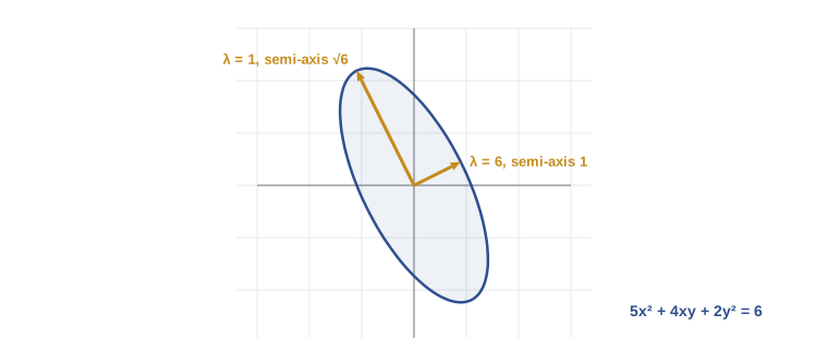
A quadratic form on \(\mathbb{R}^n\) is a function \(q(\mathbf{x}) = \mathbf{x}^{T}A\mathbf{x} = \sum_{i,j} a_{ij}x_ix_j\). We may always take \(A\) symmetric, replacing it by \((A + A^{T})/2\), which gives the same \(q\). For example \(q(x, y) = 5x^2 + 4xy + 2y^2\) has \(A = \begin{pmatrix} 5 & 2 \\ 2 & 2 \end{pmatrix}\): the cross coefficient is split equally between the two off-diagonal entries.
Theorem (principal axes). With \(A = QDQ^{T}\) and new coordinates \(\mathbf{y} = Q^{T}\mathbf{x}\),
An orthogonal change of coordinates, a rotation possibly combined with a reflection, removes every cross term. The new axes, along the eigenvectors, are the principal axes. For the example, the eigenvalues are 6 and 1 with eigenvectors \((2, 1)/\sqrt5\) and \((-1, 2)/\sqrt5\), so the curve \(q = 6\) is an ellipse with semi-axes \(1\) along \((2, 1)\) and \(\sqrt6\) along \((-1, 2)\). In general the semi-axis along \(\mathbf{q}_i\) of the ellipsoid \(q(\mathbf{x}) = 1\) is \(1/\sqrt{\lambda_i}\).
Classifying quadratic forms
A symmetric matrix \(A\), and its form, is positive definite if \(q(\mathbf{x}) > 0\) for all \(\mathbf{x} \ne \mathbf{0}\); positive semidefinite if \(q \ge 0\); negative definite or semidefinite similarly; and indefinite if \(q\) takes both signs. By the principal axes theorem, the classification is read off the signs of the eigenvalues.
| Type | Eigenvalues | Level sets of q = 1 in the plane | Other tests |
|---|---|---|---|
| Positive definite | All positive | Ellipse | All leading principal minors positive; Cholesky \(A = LL^{T}\) exists |
| Positive semidefinite | All non-negative | Pair of parallel lines or empty when degenerate | \(A = B^{T}B\) for some \(B\) |
| Indefinite | Some positive, some negative | Hyperbola | \(\det A < 0\) in the 2 by 2 case |
| Negative definite | All negative | Empty | \(-A\) positive definite |
Sylvester's criterion says \(A\) is positive definite exactly when every leading principal minor, the determinant of the top-left \(k \times k\) block, is positive. A caution: the analogous statement with non-negative minors does not characterize semidefiniteness; \(\begin{pmatrix} 0 & 0 \\ 0 & -1 \end{pmatrix}\) has leading minors 0 and 0 but is negative semidefinite. Sylvester's law of inertia adds that the numbers of positive, negative and zero eigenvalues are unchanged by any invertible congruence \(A \mapsto S^{T}AS\), not only orthogonal ones, so they are intrinsic to the form.
Every matrix of the form \(B^{T}B\) is positive semidefinite, because \(\mathbf{x}^{T}B^{T}B\mathbf{x} = \|B\mathbf{x}\|^2\), and it is positive definite exactly when \(B\) has independent columns. Covariance matrices are of this form (with \(B\) the centred data matrix divided by \(\sqrt{n - 1}\)), which is why they are always semidefinite. Conversely every positive semidefinite \(A\) has a unique positive semidefinite square root \(A^{1/2} = QD^{1/2}Q^{T}\).
Worked problem
The second derivative test
Classify the critical point at the origin of \(f(x, y) = x^2 + 3xy + y^2 + x^3\).
Show solution
- The gradient vanishes at the origin, and the Hessian there is \(H = \begin{pmatrix} 2 & 3 \\ 3 & 2 \end{pmatrix}\).
- Near the origin \(f \approx \frac12\mathbf{x}^{T}H\mathbf{x}\), a quadratic form.
- \(\det H = 4 - 9 = -5 < 0\), so the eigenvalues have opposite signs; they are 5 and \(-1\).
- The form is indefinite: \(f\) increases along \((1, 1)\) and decreases along \((1, -1)\).
Answer: The origin is a saddle point. The multivariable second derivative test is exactly the classification of the Hessian quadratic form, and in optimization for machine learning (AI-210) the eigenvalues of the Hessian set the safe learning rate.
The Rayleigh quotient
For a symmetric \(A\) with eigenvalues \(\lambda_1 \ge \lambda_2 \ge \dots \ge \lambda_n\), the Rayleigh quotient is \(R(\mathbf{x}) = \mathbf{x}^{T}A\mathbf{x}/\mathbf{x}^{T}\mathbf{x}\). In principal coordinates, \(R = \sum\lambda_iy_i^2/\sum y_i^2\) is a weighted average of the eigenvalues, so
with the maximum attained at the top eigenvector. More generally the Courant–Fischer theorem says \(\lambda_k\) is the maximum of the minimum of \(R\) over \(k\)-dimensional subspaces. The variational view is how principal component analysis is defined: the first principal component is the unit direction that maximizes the variance \(\mathbf{x}^{T}C\mathbf{x}\) of the data, where \(C\) is the covariance matrix, and so it is the top eigenvector of \(C\). In spectral graph methods the second-smallest eigenvector of a graph Laplacian, found the same way, splits a graph into two well-separated clusters, a technique used for mesh segmentation in CMPUT-411.
import numpy as np
np.set_printoptions(precision=4, suppress=True)
rng = np.random.default_rng(221)

A = np.array([[5.0, 2.0], [2.0, 2.0]])
lam, Q = np.linalg.eigh(A)
print("eigenvalues:", lam)
print("Q orthogonal:", np.allclose(Q.T @ Q, np.eye(2)))
recon = sum(l * np.outer(q, q) for l, q in zip(lam, Q.T))
print("sum of lambda q q^T recovers A:", np.allclose(recon, A))

def classify(S):
    ev = np.linalg.eigvalsh(S)
    tol = 1e-12 * max(1.0, abs(ev).max())
    pos, neg = (ev > tol).sum(), (ev < -tol).sum()
    if neg == 0:
        return "positive definite" if pos == len(ev) else "positive semidefinite"
    if pos == 0:
        return "negative definite" if neg == len(ev) else "negative semidefinite"
    return "indefinite"

tests = {
    "5x^2 + 4xy + 2y^2": A,
    "x^2 + 3xy + y^2": np.array([[1.0, 1.5], [1.5, 1.0]]),
    "x^2 + 2xy + y^2": np.array([[1.0, 1.0], [1.0, 1.0]]),
    "B^T B, B 5x3 random": (lambda B: B.T @ B)(rng.standard_normal((5, 3))),
}
for name, S in tests.items():
    print(f"{name:22s} {classify(S)}")

# Rayleigh quotient over many random unit vectors stays between the extreme eigenvalues
S = rng.standard_normal((6, 6)); S = S + S.T
ev = np.linalg.eigvalsh(S)
X = rng.standard_normal((6, 20000)); X /= np.linalg.norm(X, axis=0)
R = np.einsum("ij,ij->j", X, S @ X)
print(f"eigenvalue range [{ev[0]:.4f}, {ev[-1]:.4f}], sampled Rayleigh range [{R.min():.4f}, {R.max():.4f}]")eigenvalues: [1. 6.] Q orthogonal: True sum of lambda q q^T recovers A: True 5x^2 + 4xy + 2y^2 positive definite x^2 + 3xy + y^2 indefinite x^2 + 2xy + y^2 positive semidefinite B^T B, B 5x3 random positive definite eigenvalue range [-5.3148, 6.6091], sampled Rayleigh range [-5.1613, 6.4801]
Random sampling of the unit sphere never escapes the interval between the smallest and largest eigenvalues, and it gets close to the ends only slowly, which is why iterative methods such as the power method and the Lanczos algorithm search for the extreme directions deliberately rather than by chance.
The power method is the simplest of those iterations. Start from a random vector and repeatedly multiply by \(A\) and normalize. In principal coordinates each multiplication scales the \(i\)th component by \(\lambda_i\), so the component along the eigenvalue of largest modulus comes to dominate, at a rate set by the ratio of the two largest moduli. The Rayleigh quotient of the iterate converges to that eigenvalue twice as fast, in the sense that its error is roughly the square of the error in the direction. PageRank, mentioned in lesson 6, was computed with exactly this iteration on a matrix with billions of rows, because it needs nothing but repeated matrix–vector products.
Common mistakes
MistakeWriting the matrix of \(5x^2 + 4xy + 2y^2\) with 4 in one off-diagonal entry and 0 in the other.
InsteadUse a symmetric matrix and split the cross coefficient: 2 and 2.
MistakeAssuming a real matrix with real eigenvalues is symmetric.
Instead\(\begin{pmatrix} 1 & 1 \\ 0 & 2 \end{pmatrix}\) has real eigenvalues but non-orthogonal eigenvectors.
MistakeTesting semidefiniteness with non-negative leading principal minors.
InsteadCheck all eigenvalues, or all principal minors, not only the leading ones.
MistakeTaking the semi-axis along \(\mathbf{q}_i\) of \(\mathbf{x}^{T}A\mathbf{x} = 1\) to be \(\lambda_i\).
InsteadIt is \(1/\sqrt{\lambda_i}\).
MistakeUsing a general eigen-solver for symmetric matrices.
InsteadUse a symmetric solver such as eigh; it returns real eigenvalues and orthonormal eigenvectors.
Summary and key terms
- Self-adjoint operators have real eigenvalues and orthogonal eigenvectors for distinct eigenvalues.
- Real spectral theorem: \(A\) is symmetric exactly when \(A = QDQ^{T}\) with \(Q\) orthogonal.
- Complex spectral theorem: an operator is unitarily diagonalizable exactly when it is normal.
- A quadratic form has no cross terms in its principal axes, the eigenvectors of its symmetric matrix.
- Eigenvalue signs classify forms; Sylvester criterion and Cholesky test positive definiteness.
- The Rayleigh quotient lies between the extreme eigenvalues, and its maximizer is the top eigenvector.
- self-adjoint operator
- An operator with \(T^{*} = T\).
- spectral theorem
- Symmetric (or normal) operators have an orthonormal eigenbasis.
- normal operator
- An operator commuting with its adjoint.
- quadratic form
- A function \(\mathbf{x}^{T}A\mathbf{x}\) with \(A\) symmetric.
- principal axes
- The eigenvector directions of the matrix of a quadratic form.
- positive definite
- \(\mathbf{x}^{T}A\mathbf{x} > 0\) for every nonzero \(\mathbf{x}\).
- Rayleigh quotient
- \(\mathbf{x}^{T}A\mathbf{x}/\mathbf{x}^{T}\mathbf{x}\).
- law of inertia
- The counts of positive, negative and zero eigenvalues are invariant under congruence.
Practice problems
Work each problem on paper first, then reveal the answer to check.
Orthogonally diagonalize \(\begin{pmatrix} 2 & 2 \\ 2 & 5 \end{pmatrix}\).
Show answer
Eigenvalues 6 and 1 with unit eigenvectors \((1, 2)/\sqrt5\) and \((2, -1)/\sqrt5\).
Prove that a real symmetric matrix with all eigenvalues positive is positive definite.
Show answer
With \(\mathbf{y} = Q^{T}\mathbf{x} \ne 0\), \(\mathbf{x}^{T}A\mathbf{x} = \sum\lambda_iy_i^2 > 0\).
Classify \(x^2 + 4xy + y^2\).
Show answer
Matrix with entries 1, 2, 2, 1; eigenvalues 3 and \(-1\); indefinite.
Prove that the eigenvalues of an orthogonal matrix have modulus 1.
Show answer
\(\|Q\mathbf{v}\| = \|\mathbf{v}\|\) and \(Q\mathbf{v} = \lambda\mathbf{v}\) give \(|\lambda| = 1\).
Find the maximum of \(3x^2 + 2xy + 3y^2\) on the unit circle.
Show answer
Eigenvalues 4 and 2, so the maximum is 4, at \(\pm(1, 1)/\sqrt2\).
Prove that if \(A\) is positive definite, so is \(A^{-1}\).
Show answer
Its eigenvalues are \(1/\lambda_i > 0\) and it is symmetric.
Lesson quiz · 5 questions
Score 60% or more to complete this lesson.
Create a free account to save your progress, take quizzes and earn a certificate.