
MATH-221 · Lesson 5 of 12 · 23 min
Determinants and eigenvalues revisited
MATH-125 introduced determinants through cofactor expansion and eigenvalues through the equation \(\det(A - \lambda I) = 0\). Both were tools for computing with matrices. This lesson looks at them again from the point of view of the course: determinants as the unique function with certain structural properties, and eigenvalues as properties of a linear operator, independent of any basis. That shift in viewpoint is what makes the next three lessons possible. We prove that the determinant is characterized by three axioms, derive the product rule from that characterization rather than from computation, define eigenvalues for operators on any vector space, and prove the fundamental fact that eigenvectors for distinct eigenvalues are independent.
The determinant as an alternating multilinear form
Think of an \(n \times n\) matrix as a list of its columns \(\mathbf{a}_1, \dots, \mathbf{a}_n\). A function \(D\) of \(n\) columns in \(\mathbb{F}^n\) is called:
- multilinear if it is linear in each column when the others are held fixed;
- alternating if it is zero whenever two columns are equal;
- normalized if \(D(\mathbf{e}_1, \dots, \mathbf{e}_n) = 1\).
Theorem. There is exactly one function with all three properties, and it is the determinant. This is the cleanest definition of the determinant, because every property you know follows from it, and the cofactor formula becomes a consequence rather than a definition.
First, alternating implies antisymmetric: swapping two columns changes the sign. Proof: put \(\mathbf{a}_i + \mathbf{a}_j\) in both positions \(i\) and \(j\). By the alternating property the result is 0; expanding by multilinearity gives \(D(\dots \mathbf{a}_i \dots \mathbf{a}_i \dots) + D(\dots \mathbf{a}_i \dots \mathbf{a}_j \dots) + D(\dots \mathbf{a}_j \dots \mathbf{a}_i \dots) + D(\dots \mathbf{a}_j \dots \mathbf{a}_j \dots)\). The first and last terms vanish, so the middle two are negatives of each other.
Second, uniqueness. Write each column as \(\mathbf{a}_j = \sum_i a_{ij}\mathbf{e}_i\) and expand \(D(\mathbf{a}_1, \dots, \mathbf{a}_n)\) by multilinearity. You get a sum over all ways of choosing one standard vector for each column. Any term that chooses the same \(\mathbf{e}_i\) twice vanishes, so only permutations \(\sigma\) survive, and each such term is \(a_{\sigma(1)1}\cdots a_{\sigma(n)n} D(\mathbf{e}_{\sigma(1)}, \dots, \mathbf{e}_{\sigma(n)})\). Sorting the standard vectors back into order by swaps contributes the sign of the permutation. Hence
which is the Leibniz formula. Every alternating multilinear normalized function equals this sum, so there is at most one; and one checks that the sum does have the three properties, so there is exactly one. A useful refinement: any alternating multilinear function \(D\), normalized or not, equals \(D(I) \det\).
The product rule without computation
Theorem. \(\det(AB) = \det A \det B\). Proof: fix \(A\) and define \(D(B) = \det(AB)\) as a function of the columns of \(B\). The columns of \(AB\) are \(A\mathbf{b}_1, \dots, A\mathbf{b}_n\), so \(D\) is multilinear (because \(A\) is linear) and alternating (two equal columns of \(B\) give two equal columns of \(AB\)). By the refinement above, \(D(B) = D(I)\det B = \det A \det B\). That is the whole proof, with no index calculations at all.
Consequences follow quickly. If \(A\) is invertible then \(\det A \det A^{-1} = \det I = 1\), so \(\det A \ne 0\). Conversely, if \(A\) is singular its columns are dependent, one column is a combination of the others, and multilinearity plus the alternating property make the determinant zero. So \(A\) is invertible exactly when \(\det A \ne 0\). The transpose rule \(\det A^{T} = \det A\) follows from the Leibniz formula by re-indexing over inverse permutations, which have the same sign.
The determinant of an operator
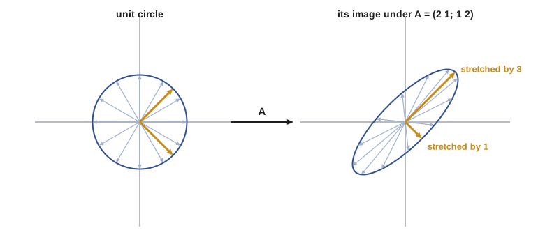
Lesson 4 showed that similar matrices have equal determinants. That lets us define the determinant of an operator \(T : V \to V\) on a finite-dimensional space as \(\det [T]_{\mathcal{B}}\) for any basis \(\mathcal{B}\): the answer does not depend on the basis. Geometrically, \(|\det T|\) is the factor by which \(T\) scales volumes, and the sign records whether it preserves or reverses orientation. For example, the transpose operator on \(M_{2 \times 2}\) is a permutation of a basis with one swap, so its determinant is \(-1\); the derivative on \(P_3\) has determinant 0 because it kills constants.
| Property | Statement | Source |
|---|---|---|
| Multilinear | Linear in each column separately | Axiom |
| Alternating | Zero when two columns agree | Axiom |
| Antisymmetric | Swapping two columns changes the sign | Follows from the axioms |
| Column operations | Adding a multiple of one column to another changes nothing | Multilinear plus alternating |
| Product rule | \(\det(AB) = \det A \det B\) | Uniqueness |
| Invertibility | \(A\) invertible exactly when \(\det A \ne 0\) | Product rule plus dependence |
| Triangular matrices | Determinant is the product of the diagonal entries | Leibniz formula |
| Basis independence | \(\det(P^{-1}AP) = \det A\) | Product rule |
Eigenvalues of an operator
Let \(T : V \to V\) be an operator on a vector space over \(\mathbb{F}\), which is \(\mathbb{R}\) or \(\mathbb{C}\). A scalar \(\lambda\) is an eigenvalue of \(T\) if there is a nonzero \(\mathbf{v}\) with \(T\mathbf{v} = \lambda\mathbf{v}\); such a \(\mathbf{v}\) is an eigenvector. The eigenspace is
which is a subspace, being a kernel. This definition makes sense in any vector space, even infinite-dimensional ones. On the space of smooth functions, the derivative has every real number as an eigenvalue: \(D(e^{\lambda t}) = \lambda e^{\lambda t}\). The shift operator on sequences, \((a_0, a_1, a_2, \dots) \mapsto (a_1, a_2, \dots)\), has eigenvectors the geometric sequences \((1, \lambda, \lambda^2, \dots)\). These examples are the theoretical root of the exponential solutions of differential equations and the power solutions of recurrences.
In finite dimensions the following are equivalent for an operator \(T\) and scalar \(\lambda\): \(\lambda\) is an eigenvalue; \(T - \lambda I\) is not injective; \(T - \lambda I\) is not surjective; \(T - \lambda I\) is not invertible; \(\det(T - \lambda I) = 0\). The middle equivalences use rank–nullity from lesson 3, which says that for an operator on a finite-dimensional space injective, surjective and invertible coincide.
The characteristic polynomial of \(T\) is \(p_T(\lambda) = \det(\lambda I - T)\), computed in any basis. It is monic of degree \(n = \dim V\), its eigenvalues are its roots in \(\mathbb{F}\), and its coefficients include two invariants you already know:
If \(p_T\) factors completely, as it always does over \(\mathbb{C}\), then \(\operatorname{tr} T\) is the sum of the eigenvalues and \(\det T\) their product, each counted with multiplicity.
Existence of eigenvalues
Theorem. Every operator on a nonzero finite-dimensional complex vector space has an eigenvalue. Proof: the characteristic polynomial has degree \(n \ge 1\) and, by the fundamental theorem of algebra, a complex root. Over \(\mathbb{R}\) this fails: rotation of the plane by \(90^\circ\) has matrix \(\begin{pmatrix} 0 & -1 \\ 1 & 0 \end{pmatrix}\) and characteristic polynomial \(\lambda^2 + 1\), with no real root. No nonzero vector is sent to a multiple of itself. This is why so much of the theory is cleanest over \(\mathbb{C}\), and why the spectral theorem of lesson 11, which guarantees real eigenvalues for symmetric matrices, is so valuable.
Over \(\mathbb{R}\), every operator on an odd-dimensional space has a real eigenvalue, because a real polynomial of odd degree has a real root. Every real operator also has an invariant subspace of dimension 1 or 2: take a complex eigenvector \(\mathbf{u} + i\mathbf{w}\), and then the real span of \(\mathbf{u}\) and \(\mathbf{w}\) is invariant. Lesson 7 develops invariant subspaces in general.
Independence of eigenvectors
Theorem. Eigenvectors \(\mathbf{v}_1, \dots, \mathbf{v}_k\) belonging to distinct eigenvalues \(\lambda_1, \dots, \lambda_k\) are linearly independent.
Proof. Suppose not, and let \(m\) be the smallest index for which \(\mathbf{v}_m\) is a combination of the earlier ones (the dependence lemma of lesson 2): \(\mathbf{v}_m = c_1\mathbf{v}_1 + \dots + c_{m-1}\mathbf{v}_{m-1}\). Apply \(T\): \(\lambda_m\mathbf{v}_m = c_1\lambda_1\mathbf{v}_1 + \dots + c_{m-1}\lambda_{m-1}\mathbf{v}_{m-1}\). Multiply the first equation by \(\lambda_m\) and subtract: \(0 = c_1(\lambda_m - \lambda_1)\mathbf{v}_1 + \dots + c_{m-1}(\lambda_m - \lambda_{m-1})\mathbf{v}_{m-1}\). The vectors \(\mathbf{v}_1, \dots, \mathbf{v}_{m-1}\) are independent by minimality of \(m\), so each \(c_i(\lambda_m - \lambda_i) = 0\), and since the eigenvalues are distinct, each \(c_i = 0\). Then \(\mathbf{v}_m = \mathbf{0}\), contradicting that it is an eigenvector.
Two corollaries matter immediately. An operator on an \(n\)-dimensional space has at most \(n\) distinct eigenvalues. And the sum of eigenspaces for distinct eigenvalues is direct: \(E_{\lambda_1} + \dots + E_{\lambda_k} = E_{\lambda_1} \oplus \dots \oplus E_{\lambda_k}\). If those eigenspaces together have dimension \(n\), we have a basis of eigenvectors, and that is the subject of lesson 6.
Two kinds of multiplicity
The algebraic multiplicity of an eigenvalue \(\lambda\) is the number of times \(\lambda\) appears as a root of \(p_T\). Its geometric multiplicity is \(\dim E_\lambda\). These can differ, and the gap between them is the whole story of the Jordan form.
Theorem. For every eigenvalue, \(1 \le \text{geometric multiplicity} \le \text{algebraic multiplicity}\). Proof: let \(g = \dim E_\lambda\) and extend a basis of \(E_\lambda\) to a basis of \(V\). In that basis the matrix of \(T\) has block form with \(\lambda I_g\) in the top-left corner, zeros below it, and some blocks \(B\) and \(C\) to the right. Its characteristic polynomial is \((x - \lambda)^g \det(xI - C)\), so \(\lambda\) is a root at least \(g\) times.
Worked problem
A matrix with a multiplicity gap
Find the eigenvalues and both multiplicities for \(A = \begin{pmatrix} 2 & 1 & 0 \\ 0 & 2 & 0 \\ 0 & 0 & 3 \end{pmatrix}\).
Show solution
- The matrix is upper triangular, so \(p_A(\lambda) = (\lambda - 2)^2(\lambda - 3)\).
- Eigenvalue 2 has algebraic multiplicity 2; eigenvalue 3 has algebraic multiplicity 1.
- \(A - 2I = \begin{pmatrix} 0 & 1 & 0 \\ 0 & 0 & 0 \\ 0 & 0 & 1 \end{pmatrix}\) has rank 2, so \(\dim E_2 = 3 - 2 = 1\), spanned by \(\mathbf{e}_1\).
- \(A - 3I\) has rank 2, so \(\dim E_3 = 1\), spanned by \(\mathbf{e}_3\).
Answer: Eigenvalue 2: algebraic 2, geometric 1. Eigenvalue 3: algebraic 1, geometric 1. The eigenvectors span only a plane, so \(A\) has no eigenvector basis.
Computing eigenvalues in practice
The characteristic polynomial is a fine theoretical tool and a poor numerical one. Roots of polynomials are extremely sensitive to their coefficients: Wilkinson's famous polynomial \((x - 1)(x - 2)\cdots(x - 20)\) has roots that move into the complex plane when one coefficient is perturbed in the tenth significant digit. Numerical libraries never form \(p_A\). They use the QR algorithm, which repeatedly factors \(A_k = Q_kR_k\) and forms \(A_{k+1} = R_kQ_k = Q_k^{T}A_kQ_k\), a sequence of similar matrices that converges toward triangular form, with the eigenvalues appearing on the diagonal. Lesson 10 builds the QR factorization; here we simply compare the two approaches.
import numpy as np
np.set_printoptions(precision=6, suppress=True)
rng = np.random.default_rng(221)

A = np.array([[2.0, 1.0, 0.0],
              [0.0, 2.0, 0.0],
              [0.0, 0.0, 3.0]])
vals, vecs = np.linalg.eig(A)
print("eigenvalues:", vals.real)
print("rank of A - 2I:", np.linalg.matrix_rank(A - 2 * np.eye(3)), "so dim E_2 =", 3 - np.linalg.matrix_rank(A - 2 * np.eye(3)))

# trace and determinant from the eigenvalues of a random matrix
B = rng.integers(-4, 5, size=(4, 4)).astype(float)
ev = np.linalg.eigvals(B)
print("trace:", np.trace(B), " sum of eigenvalues:", round(ev.sum().real, 6))
print("det:  ", round(np.linalg.det(B), 6), " product of eigenvalues:", round(np.prod(ev).real, 6))

# a few steps of unshifted QR iteration on a symmetric matrix
S = B + B.T
Ak = S.copy()
for _ in range(60):
    Q, R = np.linalg.qr(Ak)
    Ak = R @ Q
print("diagonal after QR iteration:", np.sort(np.diag(Ak)))
print("eigvalsh for comparison: ", np.linalg.eigvalsh(S))eigenvalues: [2. 2. 3.] rank of A - 2I: 2 so dim E_2 = 1 trace: 0.0 sum of eigenvalues: 0.0 det: -220.0 product of eigenvalues: -220.0 diagonal after QR iteration: [-7.086679 -5.649679 2.321409 10.414949] eigvalsh for comparison: [-7.086679 -5.649679 2.321409 10.414949]
The QR iteration recovers the eigenvalues of the symmetric matrix to six decimals without ever writing down a polynomial. Real implementations add shifts and a preliminary reduction to Hessenberg form, which make it fast and reliable; the version above shows only the idea. The same algorithm sits underneath principal component analysis in AI-210 and the eigen-solvers used for mesh processing in CMPUT-411.
Common mistakes
MistakeDefining eigenvalues only for matrices.
InsteadEigenvalues belong to the operator; every matrix of the operator has the same ones.
MistakeAssuming every real matrix has a real eigenvalue.
InsteadRotations of the plane have none; existence is guaranteed over \(\mathbb{C}\).
MistakeTaking the geometric multiplicity to equal the algebraic one.
InsteadGeometric multiplicity can be smaller; compute \(\dim\ker(A - \lambda I)\).
MistakeThinking eigenvectors for the same eigenvalue are automatically independent.
InsteadOnly eigenvectors for distinct eigenvalues are; within one eigenspace you must choose a basis.
MistakeComputing eigenvalues numerically from the roots of the characteristic polynomial.
InsteadUse a QR-based routine; polynomial roots are badly conditioned.
Summary and key terms
- The determinant is the unique normalized alternating multilinear function of the columns, and the Leibniz formula follows.
- The product rule follows from uniqueness, and the determinant of an operator is basis independent.
- Eigenvalues and eigenspaces are defined for any operator; in finite dimensions they are the roots of the characteristic polynomial.
- Every complex operator has an eigenvalue; real operators may not.
- Eigenvectors for distinct eigenvalues are independent, so eigenspaces form a direct sum.
- Geometric multiplicity is at least 1 and at most the algebraic multiplicity.
- multilinear
- Linear in each argument when the others are held fixed.
- alternating
- Zero whenever two arguments are equal.
- Leibniz formula
- The determinant as a signed sum over all permutations.
- eigenspace
- The kernel of \(T - \lambda I\).
- characteristic polynomial
- \(\det(\lambda I - T)\), monic of degree \(\dim V\).
- algebraic multiplicity
- The multiplicity of an eigenvalue as a root of the characteristic polynomial.
- geometric multiplicity
- The dimension of the eigenspace.
- QR algorithm
- An iteration of similar matrices that converges to triangular form, revealing eigenvalues.
Practice problems
Work each problem on paper first, then reveal the answer to check.
Prove that a matrix with a zero column has determinant 0 using only the axioms.
Show answer
Multilinearity in that column: \(D(\dots, 0\cdot\mathbf{x}, \dots) = 0 \cdot D(\dots, \mathbf{x}, \dots) = 0\).
Prove that \(\det(cA) = c^n \det A\) for an \(n \times n\) matrix.
Show answer
Each of the n columns is scaled by c, and multilinearity pulls out one factor c per column.
Find the eigenvalues of the transpose operator on \(M_{2 \times 2}\).
Show answer
Symmetric matrices are fixed (eigenvalue 1, dimension 3) and antisymmetric ones are negated (eigenvalue \(-1\), dimension 1).
Show that \(A\) and \(A^{T}\) have the same eigenvalues.
Show answer
\(\det(\lambda I - A^{T}) = \det((\lambda I - A)^{T}) = \det(\lambda I - A)\).
Prove that if \(T^2 = 0\) then 0 is the only eigenvalue of \(T\).
Show answer
If \(T\mathbf{v} = \lambda\mathbf{v}\) with \(\mathbf{v} \ne 0\), then \(0 = T^2\mathbf{v} = \lambda^2\mathbf{v}\), so \(\lambda = 0\).
Prove that \(AB\) and \(BA\) have the same nonzero eigenvalues.
Show answer
If \(AB\mathbf{v} = \lambda\mathbf{v}\) with \(\lambda \ne 0\), then \(B\mathbf{v} \ne 0\) and \(BA(B\mathbf{v}) = \lambda B\mathbf{v}\).
Lesson quiz · 5 questions
Score 60% or more to complete this lesson.
Create a free account to save your progress, take quizzes and earn a certificate.