
MATH-221 · Lesson 6 of 12 · 21 min
Diagonalization and applications
An operator is easiest to understand when there is a basis in which it just stretches each basis vector. Then its matrix is diagonal, its powers are diagonal, and its behaviour over time can be read off from the stretch factors. This lesson gives the exact criterion for when such a basis exists, explains how to find it, and puts it to work on three classic problems: linear recurrences such as the Fibonacci numbers, Markov chains and their long-run behaviour, and systems of linear differential equations. Each application has the same shape. A complicated coupled system becomes a set of independent one-dimensional problems once you change to the eigenvector basis.
The criterion
An operator \(T\) on an \(n\)-dimensional space \(V\) is diagonalizable if \(V\) has a basis consisting of eigenvectors of \(T\). In matrix language, \(A\) is diagonalizable if \(A = PDP^{-1}\) with \(D\) diagonal and \(P\) invertible; the columns of \(P\) are the eigenvectors and the diagonal entries of \(D\) are the matching eigenvalues, in the same order. Lesson 4 explains why: \(D = P^{-1}AP\) is the matrix of the same operator in the basis formed by the columns of \(P\).
Theorem. Let \(\lambda_1, \dots, \lambda_k\) be the distinct eigenvalues of \(T\). The following are equivalent:
- \(T\) is diagonalizable;
- \(V = E_{\lambda_1} \oplus \dots \oplus E_{\lambda_k}\);
- \(\dim E_{\lambda_1} + \dots + \dim E_{\lambda_k} = n\);
- the characteristic polynomial splits into linear factors and every eigenvalue has geometric multiplicity equal to its algebraic multiplicity.
Proof sketch. Lesson 5 showed that the sum of eigenspaces is always direct, so its dimension is the sum of the eigenspace dimensions. That sum equals \(n\) exactly when the eigenspaces fill \(V\), which is exactly when we can choose a basis of each eigenspace and combine them into a basis of eigenvectors. For the last condition, the algebraic multiplicities add to at most \(n\), with equality when the polynomial splits, and each geometric multiplicity is at most the algebraic one. So the geometric multiplicities add to \(n\) only if the polynomial splits and there is equality in every case.
Corollary. If \(T\) has \(n\) distinct eigenvalues, it is diagonalizable. Each eigenspace then has dimension at least 1 and there are \(n\) of them. The converse is false: the identity has one eigenvalue and is diagonal already.
| Matrix | Eigenvalues | Geometric multiplicities | Diagonalizable? |
|---|---|---|---|
| \(\begin{pmatrix} 2 & 1 \\ 1 & 2 \end{pmatrix}\) | 3, 1 | 1, 1 | Yes: distinct eigenvalues |
| \(\begin{pmatrix} 4 & 0 \\ 0 & 4 \end{pmatrix}\) | 4 (twice) | 2 | Yes: already diagonal |
| \(\begin{pmatrix} 4 & 1 \\ 0 & 4 \end{pmatrix}\) | 4 (twice) | 1 | No: eigenspace too small |
| \(\begin{pmatrix} 0 & -1 \\ 1 & 0 \end{pmatrix}\) | \(\pm i\) | 1, 1 over the complex numbers | Over \(\mathbb{C}\) yes; over \(\mathbb{R}\) no |
| \(D\) on \(P_3\) | 0 (four times) | 1 | No: nilpotent and nonzero |
The rotation example shows that diagonalizability depends on the field. Over \(\mathbb{R}\) its characteristic polynomial does not split, so there is no real eigenvector basis; over \(\mathbb{C}\) the eigenvectors \((1, \mp i)\) form one. The derivative example shows the other obstruction: a nonzero nilpotent operator has only the eigenvalue 0 and an eigenspace smaller than the space. Lesson 8 shows that these two obstructions are the only ones, and that every complex operator is diagonal plus nilpotent in a suitable basis.
Powers and functions of a diagonalizable matrix
If \(A = PDP^{-1}\), then \(A^2 = PDP^{-1}PDP^{-1} = PD^2P^{-1}\), and by induction
More generally, for any polynomial \(q\), \(q(A) = Pq(D)P^{-1}\), and \(q(D)\) just applies \(q\) to each diagonal entry. This lets us define functions of matrices, such as square roots of positive matrices or the exponential, by applying the function to the eigenvalues. A clean way to state this uses the spectral projections. Write \(\mathbf{v} = \mathbf{v}_1 + \dots + \mathbf{v}_k\) with \(\mathbf{v}_i \in E_{\lambda_i}\), and let \(\Pi_i\mathbf{v} = \mathbf{v}_i\). Then \(\Pi_i\Pi_j = 0\) for \(i \ne j\), \(\Pi_i^2 = \Pi_i\), \(\Pi_1 + \dots + \Pi_k = I\), and
This is the spectral decomposition. For symmetric matrices the projections are orthogonal, which is the content of the spectral theorem in lesson 11.
Application: linear recurrences
The Fibonacci numbers satisfy \(F_{k+1} = F_k + F_{k-1}\) with \(F_0 = 0\), \(F_1 = 1\). Package two consecutive terms as a vector \(\mathbf{x}_k = (F_{k+1}, F_k)\); then \(\mathbf{x}_k = A\mathbf{x}_{k-1}\) with \(A = \begin{pmatrix} 1 & 1 \\ 1 & 0 \end{pmatrix}\), so \(\mathbf{x}_k = A^k\mathbf{x}_0\).
Worked problem
A closed form for Fibonacci numbers
Diagonalize \(A = \begin{pmatrix} 1 & 1 \\ 1 & 0 \end{pmatrix}\) and derive a formula for \(F_k\).
Show solution
- \(p_A(\lambda) = \lambda^2 - \lambda - 1\), with roots \(\varphi = (1 + \sqrt 5)/2\) and \(\psi = (1 - \sqrt 5)/2\).
- An eigenvector for \(\lambda\) is \((\lambda, 1)\), since \(A(\lambda, 1) = (\lambda + 1, \lambda) = (\lambda^2, \lambda)\) using \(\lambda^2 = \lambda + 1\).
- Write \(\mathbf{x}_0 = (1, 0)\) in the eigenvector basis: \((1, 0) = \frac{1}{\sqrt 5}\big((\varphi, 1) - (\psi, 1)\big)\).
- Then \(A^k\mathbf{x}_0 = \frac{1}{\sqrt 5}\big(\varphi^k(\varphi, 1) - \psi^k(\psi, 1)\big)\); the second component is \(F_k\).
Answer: \(F_k = (\varphi^k - \psi^k)/\sqrt 5\). Since \(|\psi| < 1\), \(F_k\) is the nearest integer to \(\varphi^k/\sqrt 5\), and \(F_{k+1}/F_k \to \varphi\).
The same method handles any linear recurrence with constant coefficients: the characteristic polynomial of the companion matrix is the characteristic polynomial of the recurrence, and when its roots are distinct the solutions are combinations of their powers. Repeated roots produce terms such as \(k r^k\), which correspond to Jordan blocks (lesson 8).
Application: Markov chains
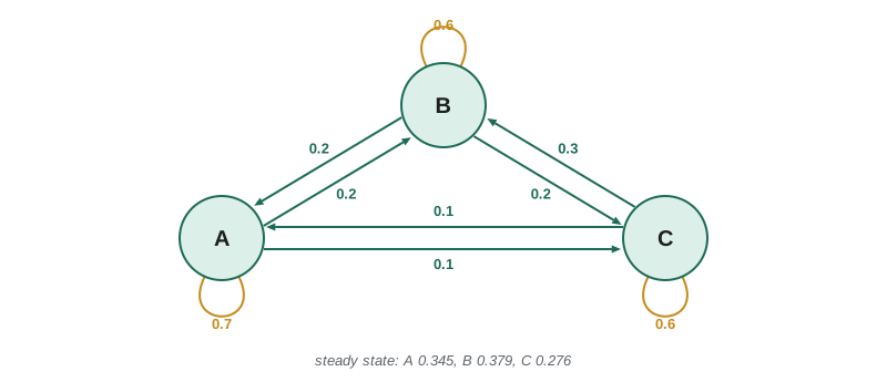
A Markov chain on \(n\) states is described by a transition matrix \(M\) whose entry \(m_{ij}\) is the probability of moving from state \(j\) to state \(i\). Each column is a probability vector, with non-negative entries adding to 1. If \(\mathbf{p}_k\) is the distribution at step \(k\), then \(\mathbf{p}_{k+1} = M\mathbf{p}_k\).
Because each column sums to 1, the row vector of ones satisfies \(\mathbf{1}^{T}M = \mathbf{1}^{T}\), so 1 is an eigenvalue of \(M^{T}\) and hence of \(M\). The Perron–Frobenius theorem says that if some power of \(M\) has all entries positive, then 1 is a simple eigenvalue, every other eigenvalue has \(|\lambda| < 1\), and the eigenvector for 1 can be scaled to a probability vector \(\boldsymbol{\pi}\), the steady state. If \(M\) is diagonalizable, write \(\mathbf{p}_0 = \boldsymbol{\pi} + c_2\mathbf{v}_2 + \dots + c_n\mathbf{v}_n\) (the coefficient of \(\boldsymbol\pi\) is 1 because all other eigenvectors have entries summing to 0); then
and the speed of convergence is governed by the second-largest \(|\lambda|\), the spectral gap. Google's original PageRank was exactly this steady state for a Markov chain on web pages.
Application: systems of differential equations
The system \(\mathbf{x}'(t) = A\mathbf{x}(t)\) couples the components of \(\mathbf{x}\). In the eigenvector basis, with \(\mathbf{x} = P\mathbf{y}\), it becomes \(\mathbf{y}' = D\mathbf{y}\): independent scalar equations \(y_i' = \lambda_iy_i\) with solutions \(y_i(t) = e^{\lambda_it}y_i(0)\). Changing back,
The matrix exponential is defined in general by the series \(e^{tA} = I + tA + t^2A^2/2! + \cdots\), which converges for every matrix; for a diagonalizable one it agrees with the formula above, term by term. The long-run behaviour is set by the real parts of the eigenvalues: if all are negative the solution decays to 0 and the equilibrium is stable; if any is positive some solutions grow. Complex eigenvalues \(a \pm bi\) produce oscillation at frequency \(b\) inside an envelope \(e^{at}\).
The code below compares the exact solution from diagonalization with the simple numerical method of Euler steps, \(\mathbf{x}_{k+1} = (I + hA)\mathbf{x}_k\), which you will meet again in numerical analysis. Euler's method is itself a matrix power, with eigenvalues \(1 + h\lambda_i\); it is stable only when those have modulus below 1, which is why it fails for large steps on stiff systems.
import numpy as np
np.set_printoptions(precision=6, suppress=True)

# Fibonacci by diagonalization versus the recurrence
A = np.array([[1.0, 1.0], [1.0, 0.0]])
vals, P = np.linalg.eig(A)
vals, P = vals.real, P.real      # the eigenvalues here are real
k = 30
Ak = P @ np.diag(vals ** k) @ np.linalg.inv(P)
fib = [0, 1]
for _ in range(k):
    fib.append(fib[-1] + fib[-2])
print("F_30 from A^30:", round(Ak[1, 0]), " from the recurrence:", fib[30])

# steady state of a three-state Markov chain (columns sum to 1)
M = np.array([[0.7, 0.2, 0.1],
              [0.2, 0.6, 0.3],
              [0.1, 0.2, 0.6]])
w, V = np.linalg.eig(M)
i = np.argmin(abs(w - 1))
pi = (V[:, i] / V[:, i].sum()).real
print("eigenvalues of M:", np.sort(w.real)[::-1])
print("steady state:", pi)
p = np.array([1.0, 0.0, 0.0])
for _ in range(40):
    p = M @ p
print("after 40 steps from state A:", p)

# x' = Ax: exact solution versus Euler steps
B = np.array([[-1.0, 2.0], [0.0, -3.0]])
lam, Q = np.linalg.eig(B)
lam, Q = lam.real, Q.real
x0 = np.array([1.0, 1.0])
t = 2.4
exact = Q @ np.diag(np.exp(lam * t)) @ np.linalg.inv(Q) @ x0
for h in (0.1, 0.01, 0.8):
    x = x0.copy()
    for _ in range(round(t / h)):
        x = x + h * (B @ x)
    print(f"Euler h={h}: {x}  error {np.linalg.norm(x - exact):.2e}")
print("exact:", exact)F_30 from A^30: 832040 from the recurrence: 832040 eigenvalues of M: [1. 0.561803 0.338197] steady state: [0.344828 0.37931 0.275862] after 40 steps from state A: [0.344828 0.37931 0.275862] Euler h=0.1: [0.159341 0.000192] error 2.14e-02 Euler h=0.01: [0.178589 0.000669] error 2.10e-03 Euler h=0.8: [ 2.76 -2.744] error 3.77e+00 exact: [0.180689 0.000747]
With \(h = 0.8\), the Euler matrix \(I + hB\) has an eigenvalue \(1 - 0.8 \times 3 = -1.4\), of modulus greater than 1, so the method oscillates and its error grows even though the true solution decays. The fix in practice is a smaller step or an implicit method; the diagnosis is pure eigenvalue analysis.
The Markov part of the output deserves a second look. The eigenvalues of \(M\) are 1, about 0.56 and about 0.34. After 40 steps the starting distribution, which put all its weight on state A, has become indistinguishable from the steady state to six decimals. That is what the formula predicts: the deviation from \(\boldsymbol\pi\) shrinks like \(0.56^{k}\), and \(0.56^{40}\) is below \(10^{-10}\). A chain whose second eigenvalue was 0.99 would need hundreds of steps for the same accuracy, so the spectral gap is the quantity to estimate before trusting a simulation of the chain. The same quantity controls how quickly Markov chain Monte Carlo methods forget their starting point, a concern you will meet in Bayesian statistics and in the sampling methods of AI-210.
When diagonalization is the wrong tool
Diagonalization is exact in theory but can be unstable in floating point. If the eigenvector matrix \(P\) is nearly singular, small errors in \(A\) produce large errors in \(P^{-1}\), and formulas like \(PD^kP^{-1}\) lose accuracy. This happens near non-diagonalizable matrices, where two eigenvectors become almost parallel. Numerical software therefore prefers the Schur form, \(A = QTQ^{*}\) with \(Q\) unitary and \(T\) upper triangular, which always exists over \(\mathbb{C}\) and uses a perfectly conditioned change of basis. For symmetric matrices the two coincide, which is one more reason the spectral theorem is so useful.
Common mistakes
MistakeConcluding that a matrix with a repeated eigenvalue cannot be diagonalized.
InsteadIt can be, provided the eigenspace is as large as the multiplicity; check \(\dim\ker(A - \lambda I)\).
MistakePutting eigenvectors in the rows of \(P\).
InsteadEigenvectors are the columns of \(P\), in the same order as the eigenvalues in \(D\).
MistakeWriting \(A^k = P^kD^kP^{-k}\).
InsteadThe inner factors cancel: \(A^k = PD^kP^{-1}\).
MistakeComputing \(e^{A}\) by exponentiating each entry of \(A\).
InsteadExponentiate the eigenvalues, or sum the power series.
MistakeAssuming any Markov chain converges to a unique steady state.
InsteadThat needs a regular chain; a chain that alternates between two states has eigenvalue \(-1\) and never settles.
Summary and key terms
- \(T\) is diagonalizable exactly when its eigenspaces have dimensions adding to \(\dim V\).
- Distinct eigenvalues guarantee diagonalizability; repeated eigenvalues need eigenspaces of full size.
- If \(A = PDP^{-1}\) then \(A^k = PD^kP^{-1}\) and \(f(A) = Pf(D)P^{-1}\).
- Linear recurrences, Markov chains and linear differential equations decouple in the eigenvector basis.
- Long-run behaviour is controlled by the eigenvalues: their moduli for powers, their real parts for exponentials.
- In floating point, ill-conditioned eigenvector matrices make diagonalization inaccurate; the Schur form is the stable alternative.
- diagonalizable
- Having a basis of eigenvectors.
- spectral projection
- The projection onto one eigenspace along the sum of the others.
- companion matrix
- The matrix that advances the state vector of a linear recurrence by one step.
- transition matrix
- A matrix of probabilities whose columns sum to 1.
- steady state
- A probability vector fixed by a transition matrix.
- matrix exponential
- \(e^{A} = \sum_k A^k/k!\).
- spectral gap
- The difference between the largest and second-largest eigenvalue moduli.
- Schur form
- A unitary similarity to an upper triangular matrix.
Practice problems
Work each problem on paper first, then reveal the answer to check.
Diagonalize \(\begin{pmatrix} 3 & 1 \\ 0 & 2 \end{pmatrix}\).
Show answer
Eigenvalues 3 and 2 with eigenvectors \((1, 0)\) and \((1, -1)\); \(P = \begin{pmatrix} 1 & 1 \\ 0 & -1 \end{pmatrix}\), \(D = \operatorname{diag}(3, 2)\).
For which \(a\) is \(\begin{pmatrix} 1 & a \\ 0 & 1 \end{pmatrix}\) diagonalizable?
Show answer
Only \(a = 0\); otherwise the eigenspace for 1 has dimension 1.
Prove that if \(A\) is diagonalizable and invertible, then \(A^{-1}\) is diagonalizable.
Show answer
\(A^{-1} = PD^{-1}P^{-1}\), and \(D^{-1}\) is diagonal since no eigenvalue is 0.
Prove that a diagonalizable matrix with \(A^2 = A\) has eigenvalues only 0 and 1.
Show answer
If \(A\mathbf{v} = \lambda\mathbf{v}\) then \(\lambda\mathbf{v} = A^2\mathbf{v} = \lambda^2\mathbf{v}\), so \(\lambda^2 = \lambda\). (In fact every such matrix is diagonalizable.)
Solve \(a_{k+1} = 5a_k - 6a_{k-1}\) with \(a_0 = 0\), \(a_1 = 1\).
Show answer
Roots 2 and 3, so \(a_k = 3^k - 2^k\).
Prove that a nilpotent diagonalizable matrix is zero.
Show answer
All its eigenvalues are 0, so \(D = 0\) and \(A = P0P^{-1} = 0\).
Lesson quiz · 5 questions
Score 60% or more to complete this lesson.
Create a free account to save your progress, take quizzes and earn a certificate.