
GEOM-440 · Lesson 9 of 12 · 21 min
Big geospatial data
The first eight lessons used datasets that fit on a laptop: a few thousand complaints, a few hundred soil samples, a season of imagery for one district. The analytics program soon outgrew that. The salinity work needs ten years of Sentinel-2 and Landsat images to see slow change; the radar archive for the coulee banks grows every twelve days; the board wants comparisons with other districts. Downloading everything and processing it locally stops working somewhere between gigabytes and terabytes. This lesson covers how geospatial data are now stored and served so that analysts can work on archives far larger than their computers, and the habits of mind that go with it.
How big is big?
Volume is the obvious dimension, but not the only one. Geospatial data are big when they are too large to move cheaply, when they arrive faster than they can be processed, or when they are spread across many sources and formats. A useful test is practical: if a task needs a person to wait for downloads, or a computer to run out of memory, the data are big for that task, and the approach must change from bringing the data to the code to bringing the code to the data.
Earth observation archives are the largest geospatial datasets most analysts touch. The Landsat archive spans more than fifty years. The Sentinel-2 pair images every land surface every five days at 10 to 60 m in thirteen bands. Agencies and cloud providers now host these archives in object storage, and increasingly in formats designed to be read in pieces over the network.
Cloud-native formats
| Format | Data | What makes it cloud-native |
|---|---|---|
| Cloud Optimized GeoTIFF (COG) | Rasters | Internal tiles and overviews, with an index at the start, so a reader can fetch just the tiles it needs by HTTP range requests |
| Zarr | Multi-dimensional arrays, such as image time series | Arrays split into compressed chunks stored as separate objects, read in parallel |
| GeoParquet | Vector tables | Columnar, compressed Parquet files with geometry columns and metadata; read only the columns and row groups needed |
| FlatGeobuf | Vector features | A spatial index at the start of the file allows bounding-box reads over HTTP |
| Cloud-optimized point cloud (COPC) | Lidar points | An octree inside a LAZ file for reads by area and level of detail |
| PMTiles | Map tiles | A single file of vector or raster tiles readable by range requests, for web maps without a tile server |
The idea common to all of them is partial reading. A COG of a full Sentinel-2 band, about 110 km on a side, is divided internally into tiles of typically 512 by 512 pixels, and the file begins with a table of where each tile lies. A reader asks the server for the header, works out which tiles cover the district, and requests only those byte ranges. Overviews, reduced-resolution copies inside the same file, let a web map show the whole scene quickly without reading full resolution.
GeoParquet stores vector data by column rather than by row, so a query that needs only field identifiers, crops and geometries skips the other forty attributes, and compression works well because each column holds one type. GeoParquet reached a stable 1.0 release in 2023 and a 1.1 release that added bounding-box columns for faster spatial filtering, and it has become a common exchange format for large vector datasets, such as national building footprints. For the district, the field table of lesson 2, with daily image statistics over ten years, is a GeoParquet file of a few hundred megabytes that GeoPandas reads in seconds.
Zarr stores arrays as chunks, and the shape of the chunks matters. A chunk of one date over a large area makes reading a whole map fast and reading one pixel's time series slow, because every date's chunk must be fetched. A chunk of many dates over a small area does the opposite. Archives built for both uses store two copies with different chunking, or choose a compromise, and the analyst should know which they are reading. GeoZarr, a convention for geospatial metadata in Zarr, is being standardized through the OGC.
Finding data: STAC
The SpatioTemporal Asset Catalog specification, STAC, describes geospatial assets in a simple, uniform way. A STAC item is a GeoJSON feature describing one acquisition: its footprint, date and time, properties such as cloud cover, and links to its assets, such as each band's COG. Items are grouped in collections and served by STAC APIs that can be searched by area, time and properties. Many public archives, including Landsat and Sentinel-2 collections on commercial clouds and on national platforms, publish STAC catalogues, so the same few lines of code search them all.
Searching a catalogue, then loading only the matching assets for the district's extent into a lazy array, is the standard pattern. Lazy means that the array is described but not read until a computation needs it, and then only the needed chunks are fetched, often in parallel by a scheduler such as Dask. An analyst can write a computation over ten years of images in a few lines, inspect its plan, and run it on a cluster of cloud machines near the data.
import pystac_client, odc.stac, planetary_computer as pc

cat = pystac_client.Client.open("https://planetarycomputer.microsoft.com/api/stac/v1", modifier=pc.sign_inplace)
items = cat.search(collections=["sentinel-2-l2a"], bbox=BBOX, datetime="2016-04-01/2026-10-31",
                   query={"eo:cloud_cover": {"lt": 30}}).item_collection()
ds = odc.stac.load(items, bands=["B04", "B08", "SCL"], bbox=BBOX, crs="EPSG:2956",
                   resolution=10, chunks={"time": 1, "x": 2048, "y": 2048})   # lazy
ndvi = ((ds.B08 - ds.B04) / (ds.B08 + ds.B04)).where(ds.SCL.isin([4, 5]))   # vegetation or bare soil only
summer = ndvi.where(ndvi.time.dt.month.isin([6, 7, 8])).groupby("time.year").median()
summer.to_zarr("district_summer_ndvi.zarr")                                  # computed chunk by chunk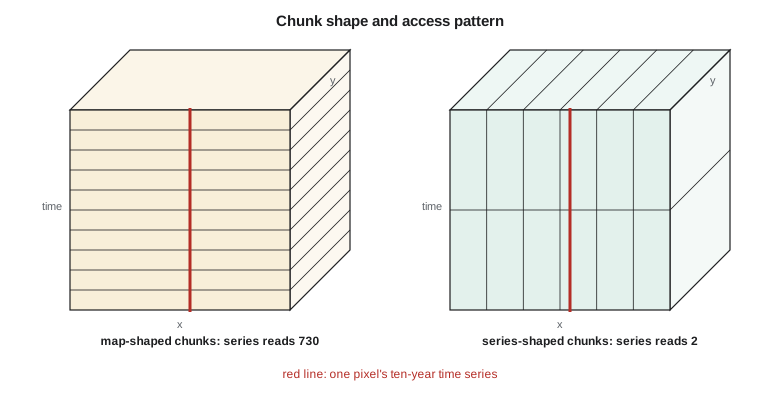
The code below does the arithmetic behind these choices. It estimates the volume of ten years of Sentinel-2 data for the district, works out how many COG tiles and bytes a district-sized read needs compared with whole scenes, compares two chunk shapes for map and time-series access, and filters a small list of STAC-like items by date, cloud cover and footprint.
import math

# 1. Volume of ten years of Sentinel-2 over the district (uint16, before compression)
area_km2 = 300.0                                    # district service area, km2
px10 = area_km2 * 1e6 / 100                         # 10 m pixels
scenes = 73 * 10                                    # 5-day revisit, ten years
bytes_total = scenes * (4 * px10 + 6 * px10 / 4 + 3 * px10 / 36) * 2
print(f"district archive: {bytes_total / 1e9:.1f} GB raw for {scenes} dates")
tile_scene = 13 * 2 * (10980 ** 2) / 1.0            # a full 110 km tile, all bands as if at 10 m
print(f"whole tiles instead: {scenes * tile_scene / 1e12:.1f} TB")

# 2. COG partial reads: 512 x 512 internal tiles over a 17 x 18 km district window
tiles = math.ceil(17000 / 10 / 512) * math.ceil(18000 / 10 / 512)
print(f"internal tiles per band read: {tiles} of {math.ceil(10980 / 512) ** 2}; "
      f"share of the file {tiles / math.ceil(10980 / 512) ** 2:.1%}")

# 3. Chunk shapes for a cube of 730 dates x 1800 x 1700 pixels
def chunks_read(shape, query):
    return math.prod(math.ceil(q / s) for q, s in zip(query, shape))
for name, shape in (("map chunks  (1, 2048, 2048)", (1, 2048, 2048)), ("series chunks (365, 128, 128)", (365, 128, 128))):
    m = chunks_read(shape, (1, 1800, 1700)); t = chunks_read(shape, (730, 1, 1))
    print(f"{name}: one map -> {m:4d} chunks, one pixel's ten-year series -> {t:4d} chunks")

# 4. Filter STAC-like items
items = [dict(id="S2A_2026-06-18", cloud=4, bbox=(-113.6, 49.4, -112.1, 50.4)),
         dict(id="S2B_2026-06-23", cloud=63, bbox=(-113.6, 49.4, -112.1, 50.4)),
         dict(id="S2A_2026-07-08", cloud=12, bbox=(-115.0, 49.4, -113.5, 50.4)),
         dict(id="S2C_2026-07-13", cloud=0, bbox=(-113.6, 49.4, -112.1, 50.4))]
aoi = (-112.95, 49.60, -112.75, 49.75)
def overlaps(a, b): return a[0] < b[2] and b[0] < a[2] and a[1] < b[3] and b[1] < a[3]
keep = [it["id"] for it in items if it["cloud"] < 30 and overlaps(it["bbox"], aoi)]
print("items to load:", keep)district archive: 24.5 GB raw for 730 dates whole tiles instead: 2.3 TB internal tiles per band read: 16 of 484; share of the file 3.3% map chunks (1, 2048, 2048): one map -> 1 chunks, one pixel's ten-year series -> 730 chunks series chunks (365, 128, 128): one map -> 210 chunks, one pixel's ten-year series -> 2 chunks items to load: ['S2A_2026-06-18', 'S2C_2026-07-13']
Ten years of the district's Sentinel-2 data come to about 25 GB before compression, a size a laptop can store but would take a long time to download and assemble. The whole tiles that contain the district would be about a hundred times more, over 2 TB, most of it fields and grassland the program does not need. A district-sized read touches 16 of the 484 internal tiles of a band, about 3 percent of the file. The chunk comparison shows the trade-off in its starkest form: with map-shaped chunks, one map is one chunk but one pixel's ten-year series needs 730; with series-shaped chunks, the series needs 2 chunks but the map needs 210. The STAC filter keeps the two items that are clear enough and actually cover the district; the cloudy item and the one from the neighbouring orbit, whose footprint misses the district, are dropped before any pixels are read.
These are back-of-envelope numbers, and that is their value. Before Theo launches a job over the archive, he works out its volume, the number of requests and the number of chunks, and compares them with what the platform can handle. A job that would touch a million chunks is redesigned before it runs, not after it fails.
Bringing code to the data
When data live in a cloud region, the cheapest and fastest computation runs in the same region. Moving data out of a cloud costs money and time; reading it from a virtual machine next to it is fast and usually free. Hosted platforms such as Google Earth Engine, Microsoft's Planetary Computer, and national services such as the Copernicus Data Space Ecosystem, run analyses on public archives without users managing servers. Each has its own terms of use, quotas and, in some cases, a proprietary programming model, so code written for one is not always portable to another. The firm's rule is to keep its core methods in open formats and open libraries, and to treat any platform as a place to run them, not a place to define them.
Scaling out has its own failure modes. Many small files are slower than a few large ones, because each request has overhead. Chunks that are too small create millions of tasks for the scheduler; chunks that are too large exhaust memory. A computation that looks parallel may hide a step that needs all the data at once, such as a global median, which then becomes the bottleneck. Profiling a small subset before launching the full job saves both money and embarrassment.
Vector data at scale
Big vector data have their own tools. Spatial indexes, such as R-trees in a database or the H3 and S2 hierarchical grids used by many cloud systems, let joins and searches skip most of the data. Spatial databases such as PostGIS, met in GEOM-330, remain the right home for transactional data that many people edit. For analysis of large tables, in-process engines such as DuckDB with its spatial extension can query GeoParquet files of hundreds of millions of rows on one machine, and cloud data warehouses offer geography types for still larger work. The choice follows the task: editing and integrity in a database, analysis in columnar files and engines built for them.
Worked problem
Choosing a chunk shape
A cube of 730 dates by 1,800 by 1,700 pixels will mostly be used to extract ten-year time series at 5,000 sample locations. Compare chunks of (1, 2048, 2048) with chunks of (365, 128, 128) for that use.
Show solution
- \[\text{map chunks: } \lceil 730/1 \rceil \times 1 \times 1 = 730 \ \text{chunks per series}\]
- \[\text{series chunks: } \lceil 730/365 \rceil \times 1 \times 1 = 2 \ \text{chunks per series}\]
- Even if nearby locations share chunks, map-shaped chunks need hundreds of reads per location; series-shaped chunks need two.
Answer: Series-shaped chunks are hundreds of times more efficient for this use; map-shaped chunks suit map display and per-date analysis.
Coulee Geomatics: the ten-year cube
Theo's pipeline builds the district's analysis cube once a week. It searches the public STAC catalogues for new Sentinel-2 and Landsat items over the district, loads only the district window from the COGs, masks clouds with the scene classification, computes indices, and appends the new dates to a Zarr store chunked for time-series access. A second copy, chunked by date, feeds the web maps. Nothing is downloaded whole, and the full ten-year cube of about the size computed above fits comfortably in the firm's cloud storage. When the board asks how the district compares with its neighbours, the same code runs with a larger bounding box.
Common mistakes
MistakeDownloading whole scenes to use a small area.
InsteadRead the area from cloud-optimized files with range requests.
MistakeChoosing chunk shapes without thinking about the main access pattern.
InsteadChunk for the dominant query, or keep two copies with different chunking.
MistakeRunning computations far from the data and moving terabytes.
InsteadCompute in the same cloud region, or on a hosted platform near the archive.
MistakeBuilding methods that only run on one proprietary platform.
InsteadKeep core methods in open formats and libraries.
Summary and key terms
- Data are big when they are too large to move cheaply or process in memory; then bring code to the data.
- COG, Zarr, GeoParquet, FlatGeobuf, COPC and PMTiles support partial reads over the network.
- Chunk shape decides whether map or time-series access is fast.
- STAC catalogues describe and serve searchable geospatial assets.
- Lazy arrays and schedulers such as Dask read only what a computation needs, in parallel.
- Columnar engines and spatial indexes handle very large vector tables.
- COG
- Cloud Optimized GeoTIFF: a tiled GeoTIFF with overviews arranged for range requests.
- Range request
- An HTTP request for a specific byte range of a file.
- Zarr
- A format storing multi-dimensional arrays as compressed chunks.
- GeoParquet
- A columnar vector format built on Apache Parquet.
- STAC
- The SpatioTemporal Asset Catalog specification for describing and searching geospatial assets.
- Lazy evaluation
- Describing a computation without performing it until results are needed.
Practice problems
Work each problem on paper first, then reveal the answer to check.
Why does a COG let a reader fetch only part of an image?
Show answer
It is internally tiled with an index at the start, so the reader requests just the tiles it needs.
What does a STAC item describe?
Show answer
One acquisition: footprint, time, properties and links to assets such as band files.
Why is GeoParquet efficient for analysis?
Show answer
It is columnar and compressed, so queries read only needed columns and row groups.
What is the risk of very small chunks?
Show answer
Millions of tiny tasks and requests, with overhead that dominates the work.
Why run analyses in the same cloud region as the data?
Show answer
Moving data out is slow and costly; local reads are fast.
Lesson quiz · 5 questions
Score 60% or more to complete this lesson.
Create a free account to save your progress, take quizzes and earn a certificate.