
GEOM-440 · Lesson 1 of 12 · 22 min
Python for geospatial data
Two winters after Coulee Geomatics built the irrigation district's GIS, the district's water manager, Marta Kowalchuk, came back with a different kind of request. The GIS now holds ten years of ditch riders' reports, 38 observation wells, the crop maps from the remote sensing program, soil samples, yield records from cooperating growers and a growing stack of radar measurements of the coulee banks. The board wants answers from all of it: where the canal leaks, where salt is building up in the soil, what drives crop yield on the district's land, and which banks are moving faster than last year. Ruth Albrecht, the firm's principal, put Leah Tran in charge of a new analytics program, with Theo Martel writing most of the code. This course follows that program. It is about turning geospatial data into defensible answers, with code that anyone can check and rerun.
What spatial data science adds
A GIS is good at storing, querying, overlaying and mapping spatial data. Spatial data science adds statistics, modelling and computation at scale. It asks how confident we can be that a cluster of wet spots is real and not chance, how to predict soil salinity between sample points with an honest estimate of the error, how to train a classifier without fooling ourselves about its accuracy, and how to process a decade of satellite images without downloading terabytes. Its tools are mostly code: scripts and notebooks that read data, transform it, analyse it and write results, so that the whole chain can be inspected and repeated.
Spatial data are different from ordinary tables in three ways that run through every lesson. First, observations near each other tend to be similar, which Tobler summed up as the first law of geography: everything is related to everything else, but near things are more related than distant things. That breaks the independence assumption behind much of classical statistics. Second, results depend on the units used to aggregate data, the modifiable areal unit problem: the same complaints counted by section, by field or by kilometre of canal can tell different stories. Third, every coordinate belongs to a coordinate reference system, and mixing systems quietly produces wrong answers.
Why Python
Python has become the common language of geospatial computing. It is free, readable, runs on every platform and sits on top of mature open-source libraries written in C and C++. Desktop GIS packages, both QGIS and the commercial systems, embed Python for scripting, so the same language moves from a one-off automation to a full analysis pipeline. R is the other strong choice, especially for spatial statistics, and much of what this course teaches carries over. The firm chose Python because Theo already used it for the GIS loading scripts, and because the deep learning and cloud tools the program needs are Python-first.
Python itself knows nothing about maps. The geospatial stack is a set of libraries that build on each other, and knowing which layer does what saves a great deal of confusion when something goes wrong.
| Library | What it does | Built on |
|---|---|---|
| GDAL/OGR | Reads and writes hundreds of raster and vector formats; reprojects and warps | C/C++ |
| PROJ (pyproj) | Coordinate reference systems and transformations, including datum grids | C/C++ |
| GEOS (Shapely) | Geometry objects and operations: intersection, buffer, union, predicates | C/C++ |
| GeoPandas | Tables whose rows have geometries; spatial joins, overlays, plotting | pandas, Shapely, pyproj |
| Rasterio | Pythonic access to raster files, windows, masks and metadata | GDAL |
| xarray, rioxarray | Labelled multi-dimensional arrays such as image time series | NumPy, Rasterio |
| PySAL (libpysal, esda, spreg, mgwr) | Spatial weights, autocorrelation, spatial regression, GWR | NumPy, SciPy |
| scikit-learn | Machine learning: classifiers, regressors, cross-validation | NumPy, SciPy |
| PyTorch | Deep learning, including convolutional networks for imagery | C++/CUDA |
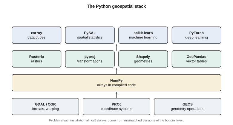
The code blocks you can run on this site use only the Python standard library, so that they work anywhere without installing anything. They implement small versions of the methods by hand, which is the best way to understand what the libraries do. Each lesson also shows listings that use the real libraries the way the firm uses them at work. The listings are marked as not run; you can run them on your own computer after installing the packages.
Data types in a geospatial program
Almost all spatial data falls into two models, met in GEOM-330. Vector data represent discrete features as points, lines and polygons with attributes: a turnout, a lateral, a field. Raster data represent continuous fields as grids of cells: a digital elevation model, a satellite band, a kriged salinity surface. Spatial data science adds two more shapes that matter. Point observations with values, such as soil samples, are the raw material of geostatistics. Arrays with a time dimension, such as a stack of images or a series of radar displacement maps, are data cubes, and they need tools built for many dimensions at once.
Inside Python, a point is ultimately a pair or triple of floating-point numbers, a polygon is a ring of such pairs, and a raster is an array with an affine transform that maps row and column to coordinates. Libraries wrap these in objects with methods, but it helps to remember the plain structures beneath, because they are what moves between programs. GeoJSON, for example, stores geometry as nested lists of longitude and latitude in a text file that any language can read.
Coordinates first
Most mistakes in spatial code are coordinate mistakes. Latitude and longitude are angles on an ellipsoid, not lengths, so distances and areas computed directly from them are wrong, and the error grows with latitude: at 50° N a degree of longitude is only about 72 km, while a degree of latitude is about 111 km. For analysis, the program projects data into a projected coordinate reference system with units of metres. The district's master system, set up in GEOM-330, is NAD83(CSRS) / UTM zone 12N, EPSG:2956, with heights in CGVD2013. Web maps and many open datasets use WGS 84 longitude and latitude, EPSG:4326, or the web Mercator system, EPSG:3857, which is fine for display and poor for measurement.
The axis order trap catches everyone once. GeoJSON and most software store longitude first, as x, then latitude, as y. The official definition of EPSG:4326 lists latitude first, and some libraries follow it. Modern pyproj lets you insist on the traditional x-then-y order with an option, and the firm's code always uses it. A dataset that lands in the Indian Ocean instead of southern Alberta has usually had its axes swapped.
The first code block reads a small table of turnouts on Lateral 7, given as latitude and longitude, and computes the distance between neighbouring turnouts three ways: treating degrees as if they were equal lengths, which is wrong; using a local equirectangular approximation that scales longitude by the cosine of latitude; and using the haversine formula on a sphere. It then writes the points as GeoJSON.
import math, json

# Turnouts on Lateral 7 as (id, latitude, longitude); positions are illustrative
BASE = (49.6450, -112.9100)
rows = [("7-10", 0.0000, 0.0000), ("7-11", 0.0021, 0.0094), ("7-12", 0.0049, 0.0183),
        ("7-13", 0.0060, 0.0291), ("7-14", 0.0087, 0.0372)]
pts = [(t, BASE[0] + a, BASE[1] + b) for t, a, b in rows]

R = 6371008.8                      # mean Earth radius, m
def naive(p, q):                   # degrees treated as equal lengths: wrong
    return math.hypot(q[1] - p[1], q[2] - p[2]) * 111195.0
def local(p, q):                   # equirectangular, scaled by cos(latitude)
    phi = math.radians((p[1] + q[1]) / 2)
    dx = math.radians(q[2] - p[2]) * math.cos(phi) * R
    dy = math.radians(q[1] - p[1]) * R
    return math.hypot(dx, dy)
def haversine(p, q):
    f1, f2 = math.radians(p[1]), math.radians(q[1])
    dl = math.radians(q[2] - p[2])
    h = math.sin((f2 - f1) / 2) ** 2 + math.cos(f1) * math.cos(f2) * math.sin(dl / 2) ** 2
    return 2 * R * math.asin(math.sqrt(h))

print("pair        naive m   local m   haversine m")
tot = 0.0
for p, q in zip(pts, pts[1:]):
    d = haversine(p, q); tot += d
    print(f"{p[0]}->{q[0]}  {naive(p, q):8.1f}  {local(p, q):8.1f}  {d:10.1f}")
print(f"lateral length along turnouts: {tot:.1f} m")

lats = [p[1] for p in pts]; lons = [p[2] for p in pts]
print("bounding box (lon, lat):", (round(min(lons), 4), round(min(lats), 4), round(max(lons), 4), round(max(lats), 4)))

fc = dict(type="FeatureCollection", features=[
    dict(type="Feature", properties=dict(turnout=t),
         geometry=dict(type="Point", coordinates=[round(lon, 6), round(lat, 6)]))  # x = lon first
    for t, lat, lon in pts])
text = json.dumps(fc)
print("GeoJSON characters:", len(text))
print("first feature:", json.dumps(fc["features"][0]))pair naive m local m haversine m
7-10->7-11 1071.0 715.9 715.9
7-11->7-12 1037.5 712.4 712.4
7-12->7-13 1207.1 787.1 787.1
7-13->7-14 949.4 655.9 655.9
lateral length along turnouts: 2871.3 m
bounding box (lon, lat): (-112.91, 49.645, -112.8728, 49.6537)
GeoJSON characters: 659
first feature: {"type": "Feature", "properties": {"turnout": "7-10"}, "geometry": {"type": "Point", "coordinates": [-112.91, 49.645]}}The naive method overstates distances by up to half, because it treats a degree of longitude as if it were as long as a degree of latitude. The local approximation and the haversine formula agree to well under a metre over these short hops, which is why the local method is common in quick scripts. For anything that must match survey control, the firm projects into the district's system with PROJ, which uses the ellipsoid and the published transformation rather than a sphere. Note too that the GeoJSON coordinates are written longitude first.
The same task with the standard libraries
At work, Theo would not write the haversine formula himself. He would read the turnouts into a GeoDataFrame, declare their coordinate system, project them and let the library compute lengths. The listing below shows that pattern. Every analysis script in the program begins this way: read, declare or check the coordinate system, project to the master system, and only then measure.
import geopandas as gpd
from shapely.geometry import LineString

turnouts = gpd.read_file("lateral7_turnouts.geojson")     # stored as EPSG:4326
assert turnouts.crs.to_epsg() == 4326
t = turnouts.to_crs(epsg=2956)                            # NAD83(CSRS) / UTM zone 12N
line = LineString(list(t.geometry))                       # turnouts in order along the lateral
print(round(line.length, 1), "m along the turnouts")
t.to_file("lateral7_turnouts.gpkg", layer="turnouts", driver="GPKG")
Environments and installation
Geospatial libraries depend on compiled C and C++ code, and mismatched versions of GDAL or PROJ are the most common reason a script works on one computer and fails on another. The firm installs its stack from the conda-forge channel, which builds GDAL, PROJ, GEOS and the Python packages to work together, and keeps one environment per project, described in a short file that lists the packages and versions. Lesson 12 returns to environments as part of reproducible work. For now, the rule is simple: never install geospatial packages into the computer's system Python, and write down what you installed.
Notebooks and scripts both have a place. A notebook mixes code, output, maps and notes, which suits exploration and teaching; the lessons here are written in that spirit. A script or a package of functions suits anything that will run more than once, because it can be tested, version-controlled and called from a pipeline without someone clicking through cells in the right order. Leah's rule for the program is that exploration happens in notebooks, but anything that produces a number for the district moves into a script with a test.
Thinking in arrays
Spatial data science handles millions of values. Python loops are slow, roughly a hundred times slower than the same arithmetic done in compiled code, so the libraries work on whole arrays at once. NumPy, under all of them, applies an operation to every element of an array in compiled code. A normalized difference vegetation index over a satellite scene is one line: subtract the red array from the near-infrared array and divide by their sum. The habit to develop is to describe the operation on the whole grid or table rather than writing a loop over cells or rows. The runnable blocks on this site use loops because they must avoid NumPy, and they are kept small for that reason.
Worked problem
How long is a degree of longitude?
How long is one degree of longitude at Lethbridge, latitude 49.70° N, on a sphere of radius 6,371 km? How does that compare with a degree of latitude?
Show solution
- \[L_\lambda = \frac{\pi}{180}\,R\cos\varphi = 0.0174533 \times 6\,371\,000 \times \cos 49.70^\circ\]
- \[L_\lambda = 111\,195 \times 0.6468 = 71\,920\ \text{m}\]
- \[L_\varphi = \frac{\pi}{180}\,R = 111\,195\ \text{m}\]
Answer: About 71.9 km, roughly 65 percent of a degree of latitude; treating the two as equal overstates east-west distances by about half.
Coulee Geomatics: the program's first rules
Leah's first memo to the team sets four rules that the rest of the course will justify. Every dataset in the program carries its coordinate system and its source, and nothing is analysed in longitude and latitude. Every result that goes to the district comes with a measure of uncertainty, even a rough one. Every model is tested on data it did not see, and the test respects space, so that nearby points are not used to check each other. And every number in a report can be regenerated from raw data by running the code. Marta asks why the last rule matters. Leah's answer is that in two years someone will ask why a recommendation was made, and the code is the only complete record of how.
Common mistakes
MistakeComputing distances or areas directly in degrees of longitude and latitude.
InsteadProject into a coordinate system with linear units, or use geodesic methods on the ellipsoid.
MistakeAssuming every file uses longitude first.
InsteadCheck the axis order; force x-then-y in pyproj and confirm data plot where expected.
MistakeInstalling geospatial packages into the system Python with mismatched GDAL versions.
InsteadUse a project environment from one consistent channel and record the versions.
MistakeWriting loops over millions of cells.
InsteadExpress the operation on whole arrays so it runs in compiled code.
Summary and key terms
- Spatial data science adds statistics, modelling and computation at scale to GIS.
- Spatial dependence, the modifiable areal unit problem and coordinate systems shape every analysis.
- The Python stack layers GeoPandas, Rasterio, xarray, PySAL and scikit-learn over GDAL, PROJ and GEOS.
- Degrees of longitude shrink with latitude; measure only in projected or geodesic terms.
- Keep one environment per project from a consistent channel, and record it.
- Explore in notebooks; move anything that produces reported numbers into tested scripts.
- Tobler's first law
- Near things are more related than distant things.
- MAUP
- The modifiable areal unit problem: results that change with the size and shape of aggregation units.
- CRS
- Coordinate reference system: the datum, coordinate system and projection that give coordinates meaning.
- GeoDataFrame
- A GeoPandas table whose rows carry geometries and a coordinate system.
- Data cube
- A multi-dimensional array, such as x, y, band and time, of gridded observations.
- Haversine formula
- A formula for great-circle distance on a sphere from latitudes and longitudes.
Practice problems
Work each problem on paper first, then reveal the answer to check.
Why is a distance computed from raw degree differences wrong at mid-latitudes?
Show answer
A degree of longitude is shorter than a degree of latitude by the cosine of latitude.
Which library performs coordinate transformations under GeoPandas?
Show answer
PROJ, through pyproj.
A dataset plots in the Indian Ocean. What is the likely cause?
Show answer
Longitude and latitude have been swapped.
Why does the program keep one environment per project?
Show answer
So that compiled libraries such as GDAL and PROJ have matching versions and results can be reproduced.
What does the modifiable areal unit problem warn about?
Show answer
Results can change when the same data are aggregated by different units.
Lesson quiz · 5 questions
Score 60% or more to complete this lesson.
Create a free account to save your progress, take quizzes and earn a certificate.