Working with vector and raster data

The analytics program needs a single table to start from: one row per field, with its crop, its area, its irrigation turnout, its average vegetation index through the season and its soil samples. Those numbers live in different places and different shapes. Field boundaries and turnouts are vectors in the GIS; vegetation indices are rasters from the remote sensing program; soil samples are points in a spreadsheet. This lesson covers the operations that move information between them: spatial joins, overlays and dissolves for vectors; windows, masks, resampling and reprojection for rasters; and zonal statistics and rasterization to cross between the two.

Vector operations as table operations

GeoPandas treats a layer as a table with a geometry column, so most vector work looks like ordinary data manipulation with a spatial condition added. A spatial join attaches attributes from one layer to another where geometries meet a predicate: each turnout gets the field it lies in, each complaint gets the nearest canal segment. Overlay operations, such as intersection, union and difference, cut polygons against each other and carry attributes from both, as when field boundaries are intersected with soil map units to find the area of each soil in each field. A dissolve merges features that share an attribute value, such as all fields of one water user, into one geometry and aggregates their attributes.

The predicates that drive joins come from the DE-9IM model of spatial relationships: intersects, within, contains, touches, crosses, overlaps. Choosing the right one matters. A turnout on the shared boundary of two fields intersects both, but is within neither if it lies exactly on the line; a join on within would drop it. For points that might sit on edges, the firm joins on intersects and resolves duplicates explicitly, keeping a record of each tie.

Joins by distance need care too. A nearest join finds, for each feature, the closest feature in another layer, and should always return the distance so that implausible matches can be filtered. A complaint 2 km from any canal is not a canal seepage complaint, however the nearest join labels it. The geometry must be in a projected system before distances are computed, as lesson 1 stressed.

import geopandas as gpd

fields = gpd.read_file("district.gpkg", layer="fields").to_crs(2956)
turnouts = gpd.read_file("district.gpkg", layer="turnouts").to_crs(2956)
soils = gpd.read_file("soil_units.gpkg").to_crs(2956)

# which field does each turnout serve? (intersects keeps points on boundaries)
tj = gpd.sjoin(turnouts, fields[["field_id", "geometry"]], how="left", predicate="intersects")
ties = tj[tj.index.duplicated(keep=False)]           # turnouts on a shared boundary
print(len(ties), "turnouts touch two fields; resolve by hand")

# area of each soil unit in each field, in hectares
parts = gpd.overlay(fields, soils, how="intersection")
parts["ha"] = parts.area / 10_000
table = parts.pivot_table(index="field_id", columns="soil_unit", values="ha", aggfunc="sum")

# one geometry per water user
users = fields.dissolve(by="user_id", aggfunc={"ha": "sum"})

Valid geometry and topology

Operations on polygons assume the polygons are valid: rings closed, no self-intersections, holes inside their shells, and rings that do not cross each other. Data digitized by hand, converted from CAD or simplified for the web often break those rules. A field boundary traced from a 1950s drawing may cross itself where the line doubled back, forming a bow tie whose area the shoelace formula computes as the difference of two lobes. Overlays on invalid geometry fail outright or, worse, return results that look plausible and are wrong.

The program checks validity on every load. Shapely reports why a geometry is invalid, and its make_valid function repairs most problems by splitting self-intersecting rings into valid parts. Repairs are logged, not silent, because a repaired bow tie may still be the wrong shape. Topology rules from GEOM-330, such as fields that must not overlap and must tile the district without gaps, are tested by overlaying the layer with itself and listing any slivers larger than a tolerance. Slivers under about a square metre are usually digitizing noise along shared edges; larger ones are real disagreements that someone with local knowledge must resolve.

Precision matters for joins as well. Coordinates stored to the millimetre in one layer and to the centimetre in another rarely meet exactly, so a point that should lie on a line tests as just off it. Snapping coordinates to a common grid, or testing within a small distance tolerance instead of exact contact, avoids a class of puzzling empty results.

Rasters: arrays with a georeference

A raster file holds one or more bands, each an array of cell values, plus the information that ties the array to the ground. The affine transform gives the coordinates of the upper-left corner and the cell size, and so maps any row and column to x and y. The coordinate reference system says what x and y mean. A nodata value marks cells with no valid measurement, such as cloud in an optical image. Forgetting the nodata value is a classic error: a mean that includes thousands of cells of −9999 is not a mean of anything.

The equation gives the centre of the cell in row r and column c, for a north-up raster with upper-left corner at x₀, y₀ and cell sizes Δx and Δy. The minus sign appears because rows count downward while northings increase upward. Rotated rasters add two more terms to the transform, but almost all analysis rasters are north-up.

Large rasters are read in windows rather than whole. A Sentinel-2 scene at 10 m has about 120 million cells per band; the district covers a small part of it. Rasterio reads just the window that covers the district, which saves memory and time, and lesson 9 shows how cloud-optimized files let it read that window over the internet without downloading the rest.

Cell values have a data type, and choosing it well keeps files small and correct. A vegetation index between −1 and 1 can be stored as a 16-bit integer scaled by 10,000, which halves the size of a 32-bit float file; a crop class map needs only an 8-bit integer. Scaled integers need the scale factor and offset recorded in the metadata, or a later user will read 4,512 where the true value is 0.4512. Lossless compression, such as DEFLATE or LZW with a predictor, typically shrinks analysis rasters by half or more at no cost in accuracy.

Resampling and reprojection

Combining rasters usually means bringing them onto one grid: the same coordinate system, cell size and alignment. Resampling chooses values for the new cells. Nearest neighbour keeps original values and is the only correct choice for categories, such as a crop class map, because averaging the codes for wheat and canola produces a class that does not exist. Bilinear and cubic resampling interpolate smoothly and suit continuous variables such as elevation or reflectance. Averaging, or mode for categories, suits aggregation to coarser cells.

Reprojecting a raster always resamples it, because the new grid does not line up with the old one. Each reprojection softens the data a little. The program's rule is to reproject each source once, directly to the master grid, rather than through intermediate systems, and to record the resampling method in the metadata.

Crossing between vector and raster

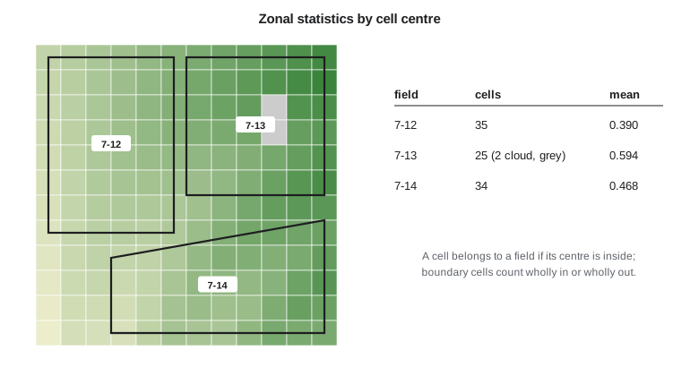
Zonal statistics summarize raster values within polygons: the mean vegetation index of each field, the maximum slope in each parcel, the share of each crop class in each section. The usual rule assigns a cell to a polygon if the cell's centre lies inside it. That rule is fast but approximate, because cells cut by the boundary count fully or not at all. For small polygons relative to the cell size the error matters; a 2 ha field covered by 10 m cells has about 200 cells, of which perhaps 50 straddle the edge. Some tools weight boundary cells by the fraction of their area inside the polygon, which is slower but more accurate.

Rasterization goes the other way, burning polygon or line attributes into a grid, as when field identifiers are written into a raster aligned with the imagery so that every pixel knows its field. Vectorization turns regions of a classified raster into polygons. Both lose information at the edges, and both should be done on the master grid with the cell size recorded.

The code below builds a small vegetation-index raster with a known transform, defines three fields as polygons, assigns cells to fields by the point-in-polygon test of their centres, and computes zonal statistics, skipping nodata cells. The point-in-polygon test is the ray-casting method: count how many polygon edges a horizontal ray from the point crosses; an odd count means inside.

import math

# A 12 x 12 vegetation index raster: upper-left corner, 20 m cells (illustrative)
X0, Y0, DX = 380000.0, 5507240.0, 20.0
NODATA = -9999.0
grid = [[round(0.35 + 0.035 * c - 0.012 * r + 0.04 * math.sin(r * c / 7.0), 3) for c in range(12)] for r in range(12)]
grid[2][9] = grid[3][9] = NODATA          # cloud
def mid(r, c): return (X0 + (c + 0.5) * DX, Y0 - (r + 0.5) * DX)

def inside(p, poly):                       # ray casting
    x, y = p; n = len(poly); ins = False
    for i in range(n):
        (x1, y1), (x2, y2) = poly[i], poly[(i + 1) % n]
        if (y1 > y) != (y2 > y) and x < x1 + (y - y1) * (x2 - x1) / (y2 - y1):
            ins = not ins
    return ins
def area(poly):                            # shoelace formula, m2
    return abs(sum(x1 * y2 - x2 * y1 for (x1, y1), (x2, y2) in zip(poly, poly[1:] + poly[:1]))) / 2

fields = {"7-12": [(380010, 5507230), (380110, 5507230), (380110, 5507090), (380010, 5507090)],
          "7-13": [(380120, 5507230), (380230, 5507230), (380230, 5507120), (380120, 5507120)],
          "7-14": [(380060, 5507070), (380230, 5507100), (380230, 5507010), (380060, 5507010)]}
AF = 1.0                                  # area units per ha
print("field  area ha  cells  nodata  mean    min    max")
for f, poly in fields.items():
    vals, nd = [], 0
    for r in range(12):
        for c in range(12):
            if inside(mid(r, c), poly):
                v = grid[r][c]
                if v == NODATA: nd += 1
                else: vals.append(v)
    a = area(poly) / 10000 * AF
    print(f"{f}   {a:7.2f}   {len(vals) + nd:5d}  {nd:6d}  {sum(vals) / len(vals):.3f}  {min(vals):.3f}  {max(vals):.3f}")
    cell_area = len(vals + [0] * nd) * DX * DX / 10000 * AF
    print(f"        cells cover {cell_area:.2f} ha ({100 * (cell_area / a - 1):+.0f}% vs polygon)")

field  area ha  cells  nodata  mean    min    max
7-12      1.40      35       0  0.390  0.266  0.502
        cells cover 1.40 ha (+0% vs polygon)
7-13      1.21      25       2  0.594  0.464  0.728
        cells cover 1.00 ha (-17% vs polygon)
7-14      1.27      34       0  0.468  0.283  0.620
        cells cover 1.36 ha (+7% vs polygon)

The comparison line under each field shows the price of the centre rule. Field 7-12 happens to line up with the grid, so its cells cover exactly its area. The other two do not: the cells counted inside 7-13 cover 17 percent less than the polygon and those inside 7-14 cover 7 percent more, because boundary cells are counted wholly in or wholly out. For a field-level mean of a smooth variable that matters little; for an area estimate it matters a great deal, which is why the program takes field areas from the polygons, never from cell counts. Field 7-13 also shows the nodata handling: its two cloudy cells are reported but kept out of the statistics.

import rasterio
from rasterio.mask import mask
import geopandas as gpd

fields = gpd.read_file("district.gpkg", layer="fields")
with rasterio.open("ndvi_2026-07-14.tif") as src:            # one band, master grid
    fields = fields.to_crs(src.crs)
    out = []
    for fid, geom in zip(fields.field_id, fields.geometry):
        arr, _ = mask(src, [geom], crop=True, filled=False)  # masked array, nodata hidden
        out.append((fid, float(arr.mean()), int(arr.count())))

Coulee Geomatics: the field table

Theo's first deliverable is the field table, rebuilt every night from the GIS and the latest imagery. Each row has the field identifier, water user, crop from the classified map by majority of cells, area from the polygon, turnout from the spatial join, mean, median and count of valid cells of the vegetation index for each image date, and the soil samples inside the field. The script logs every tie in the turnout join and every field whose valid-cell count falls below a threshold, so that Leah can see where clouds or tiny fields make the averages weak. Marta's staff open the table in a spreadsheet; the analysts read it directly into the models of the coming lessons.