Spatiotemporal analysis

Two questions from the board are about change over time. The first is about the coulee banks: the radar monitoring started in GEOM-320 showed two cracked sections moving towards the canal at 15 to 20 mm a year, and a drainage blanket and regrading were built on one of them last autumn. Has the movement slowed? The second is about the canal lining approved in lesson 4: once the leaking reach is lined next spring, will the water table in the nearby observation wells fall, and how will anyone know that the lining caused it rather than a dry year? Both questions need data indexed by place and time together, and methods that respect both kinds of dependence.

Space-time data structures

Spatiotemporal data come in a few shapes. A data cube, as in lesson 9, holds a regular grid at regular times: every pixel of every image. Panel data hold repeated measurements at fixed sites, such as monthly water levels at 38 wells or the displacement of radar scatterers every twelve days. Trajectories hold moving objects, such as a ditch rider's GPS track or a tractor's yield monitor. Event data hold things that happen at a place and time, such as the complaints of lesson 3, now with dates. Each shape has its tools: xarray for cubes, tables with site and time keys for panels, specialized libraries for trajectories, and space-time point process methods for events.

Time brings its own dependence. Values close in time are similar, just as values close in space are, and seasonal cycles add structure: water tables rise every irrigation season and fall in winter; radar displacements show seasonal swelling and shrinking of clay. A trend estimated without accounting for the season, or a test that treats monthly values as independent, misleads in the same way that ignoring spatial autocorrelation does.

Decomposing a time series

The first step with any series is to separate its parts: a long-term trend, a seasonal cycle, abrupt changes and the remainder. A simple and robust model for a displacement or water-level series fits a linear trend plus annual and semi-annual sine and cosine terms by least squares, the same trajectory model used for GNSS stations in GEOM-430. More flexible methods, such as STL decomposition, let the seasonal shape change slowly over the years. Breakpoint methods such as BFAST search for dates where the trend or the seasonal pattern changes, which is how deforestation or a new irrigation system shows up in an image time series.

Robust trends: Mann-Kendall and Theil-Sen

When the form of a trend is unknown and the data contain outliers, rank-based methods are safer than least squares. The Mann-Kendall test counts, over all pairs of observations, how many later values are higher than earlier ones and how many are lower. A strong excess of increases or decreases indicates a monotonic trend. The Theil-Sen estimator gives its size: the median of the slopes between all pairs of points. One wild value moves the median hardly at all, while it can drag a least-squares line noticeably.

Both assume independent observations. With seasonal or autocorrelated data the variance of S is too small and the test too eager, so seasonal Mann-Kendall tests compare each season only with the same season in other years, and corrected versions inflate the variance for autocorrelation. For pixel time series, applying these tests to every pixel creates the multiple-testing problem of lesson 4 again, now across millions of pixels.

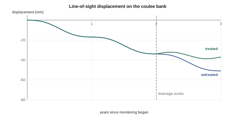
The code below simulates displacement series every twelve days over three years for a point on the untreated section and a point on the treated one, with seasonal swelling and a few outliers from unwrapping errors. For each, it applies the Mann-Kendall test and the Theil-Sen estimator to the year before the works and the year after, and compares the Theil-Sen slopes with ordinary least squares.

import math, random
random.seed(10)
t = [i * 12 / 365.25 for i in range(92)]                 # 12-day acquisitions over about three years
WORKS = 2.0                                              # drainage works on the treated section, years
def series(treated):
    d = []
    for ti in t:
        v = -17.0 * ti if not treated or ti < WORKS else -17.0 * WORKS - 3.0 * (ti - WORKS)
        d.append(v + 2.5 * math.sin(2 * math.pi * ti) + random.gauss(0, 1.2))
    for k in (20, 55, 77): d[k] += random.choice((-1, 1)) * 14.0       # unwrapping outliers
    return d

def mk(x):
    n = len(x); S = sum((x[j] > x[i]) - (x[j] < x[i]) for i in range(n) for j in range(i + 1, n))
    var = n * (n - 1) * (2 * n + 5) / 18
    z = (S - 1) / math.sqrt(var) if S > 0 else (S + 1) / math.sqrt(var) if S < 0 else 0.0
    return S, z
def sen(tt, x):
    sl = sorted((x[j] - x[i]) / (tt[j] - tt[i]) for i in range(len(x)) for j in range(i + 1, len(x)))
    m = len(sl); return sl[m // 2] if m % 2 else (sl[m // 2 - 1] + sl[m // 2]) / 2
def ols(tt, x):
    mt = sum(tt) / len(tt); mx = sum(x) / len(x)
    return sum((a - mt) * (b - mx) for a, b in zip(tt, x)) / sum((a - mt) ** 2 for a in tt)

for name, tr in (("untreated", False), ("treated", True)):
    d = series(tr)
    for label, lo, hi in (("year before works", 1.0, 2.0), ("year after works", 2.0, 3.1)):
        idx = [i for i, ti in enumerate(t) if lo <= ti < hi]
        tt = [t[i] for i in idx]; x = [d[i] for i in idx]
        S, z = mk(x)
        print(f"{name:9s} {label:17s} n={len(x):2d}  S={S:5d}  z={z:6.2f}  "
              f"Theil-Sen {sen(tt, x):6.1f} mm/yr  OLS {ols(tt, x):6.1f} mm/yr")

untreated year before works n=30  S= -381  z= -6.78  Theil-Sen  -22.2 mm/yr  OLS  -23.4 mm/yr
untreated year after works  n=31  S= -383  z= -6.49  Theil-Sen  -21.6 mm/yr  OLS  -21.5 mm/yr
treated   year before works n=30  S= -321  z= -5.71  Theil-Sen  -22.3 mm/yr  OLS  -20.7 mm/yr
treated   year after works  n=31  S= -207  z= -3.50  Theil-Sen   -6.7 mm/yr  OLS   -6.6 mm/yr

Every window shows a highly significant downward trend, because each point is still moving. The useful comparison is between slopes. On the untreated section the Theil-Sen velocity is about −22 mm a year both before and after the works date, as it should be, since nothing was done there. On the treated section it falls from about −22 to about −7 mm a year: the drainage works have cut the movement by roughly two-thirds in their first year. The Theil-Sen and least-squares slopes agree within a couple of millimetres a year in most windows; where they differ most, in the year before the works, the window contains one of the unwrapping outliers, a 14 mm jump that pulls the least-squares line by a millimetre or two but barely moves the median of 435 pairwise slopes. With real radar data, where outliers can be more frequent and larger, the difference grows, and the robust estimate is the one the firm reports.

There is a lesson in the numbers too. The simulation's true velocity before the works is −17 mm a year, yet both estimators report about −22. The extra 5 mm a year is the seasonal swelling: a one-year window that starts in one phase of the seasonal cycle and ends in another picks up part of the cycle as trend. Comparing windows of the same length and season, as the code does, cancels most of the bias in the before-after difference, but the absolute velocities are biased. Fitting the trend and the seasonal terms together, as in the decomposition model above, or using several years per window, removes it.

Before-after control-impact designs

The canal lining question is about cause, and causal questions in space and time need a design, not just a trend test. If the water table near the lined reach falls after lining, the fall could come from the lining, from a dry year, from less irrigation upstream or from all three. A before-after control-impact design, BACI, measures the same quantity before and after the intervention at impact sites, wells near the lined reach, and at control sites, similar wells near unlined reaches. The estimate of the effect is the difference in differences: the change at impact sites minus the change at control sites.

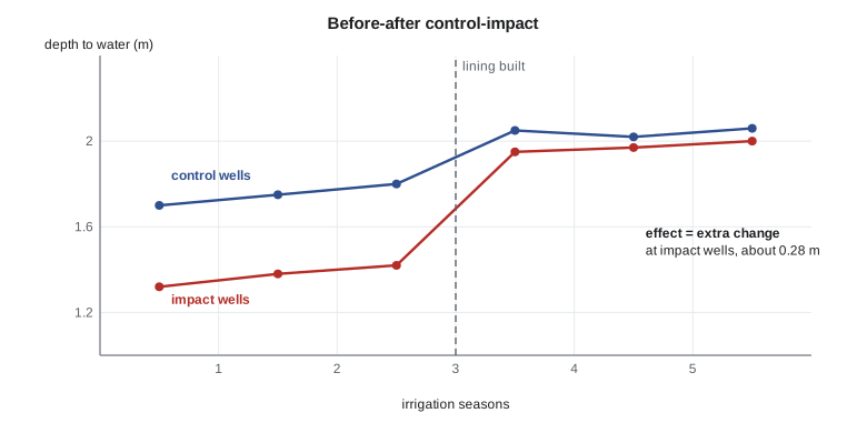
The design removes changes shared by all sites, such as weather, and leaves the change specific to the impact sites. It rests on an assumption, parallel trends: without the lining, impact and control wells would have changed alike. That is checked by comparing their behaviour in several years before the intervention. Control sites should be far enough from the impact to be unaffected, which for groundwater means outside the zone the lining could influence, but close enough to share weather and soils. Several years of data before and after, rather than one season, make the estimate far more robust, which is why the board's request in lesson 4 for a design came before the lining was built, not after.

Space-time clusters and emerging hot spots

Event data in space and time ask whether events cluster in both together: complaints that bunch in one place in one season, beyond what their spatial and temporal patterns separately would produce. The Knox test counts pairs of events close in both space and time and compares the count with permutations that shuffle the dates. Space-time scan statistics search over cylinders of varying radius and duration for the most unusual concentration. Emerging hot spot analysis, available in desktop GIS, computes Gi* for each cell of a space-time cube and then classifies each location's sequence of results as new, intensifying, persistent, diminishing or sporadic hot spots, a useful summary for maps if its many tests are kept in mind.

import xarray as xr, numpy as np
from scipy.stats import kendalltau

d = xr.open_zarr("insar_los_displacement.zarr")["los_mm"]         # time, y, x
d = d.chunk({"time": -1, "y": 256, "x": 256})
t_years = (d.time - d.time[0]) / np.timedelta64(1, "D") / 365.25
fit = d.polyfit(dim="time", deg=1)                                  # least-squares velocity per pixel
def tau(y):                                                         # Kendall's tau per pixel (rank trend)
    ok = np.isfinite(y)
    return kendalltau(np.arange(ok.sum()), y[ok])[0] if ok.sum() > 10 else np.nan
tau_map = xr.apply_ufunc(tau, d, input_core_dims=[["time"]], vectorize=True, dask="parallelized",
                         output_dtypes=[float])

Coulee Geomatics: monitoring that answers questions

Leah's monitoring plan for the next three years follows from the lesson. The radar scatterers on both bank sections are analysed every quarter with seasonal Mann-Kendall tests and Theil-Sen velocities, and the report shows each section's velocity before and after the works with confidence intervals from a block bootstrap that respects autocorrelation. Twelve observation wells, six near the reach to be lined and six near similar unlined reaches, are logged automatically every hour from this autumn, giving a full season of data before the lining and three after. Marta asks whether all this is needed to know whether the lining worked. Leah's answer is that without the control wells, a dry summer would make any lining look successful, and a wet one would make it look like a waste of money.