
GEOM-340 · Lesson 4 of 12 · 23 min
Conic projections
Canada's national maps, many provincial thematic maps and the climate and agricultural atlases that the district's agronomist reads every season are drawn on conic projections. A cone suits the middle latitudes: placed over the globe like a lampshade, it touches or cuts the Earth along parallels in the latitudes where most land lies. This lesson develops the Lambert conformal conic, the conic used for surveying and navigation, and the Albers equal-area conic, the conic used for statistics, and shows how the choice of standard parallels controls their distortion.
The geometry of a cone
When a cone is cut along one of its straight lines and unrolled, it becomes a sector of a circle. Meridians become straight lines radiating from the apex of the sector, and parallels become arcs of circles centred on the apex. The angle between two meridians on the map is not their difference in longitude but a fraction of it,
where \(n\), the cone constant, lies between 0 and 1. A cone constant of 1 gives a plane (an azimuthal projection centred on the pole) and a cone constant of 0 gives a cylinder, so the conic family sits between the other two. The radius \(\rho\) of each parallel's arc depends on latitude through a function that sets the projection's property, just as \(F(\varphi)\) did for cylinders. Map coordinates follow from polar coordinates around the apex:
where \(\rho_0\) is the radius of the parallel through the false origin and \(E_0\), \(N_0\) the false easting and northing. Because \(\theta\) depends only on longitude, the grid convergence, the angle between grid north and true north, is simply \(\theta\) itself: it is zero on the central meridian and grows in proportion to the longitude difference, west negative and east positive in the convention used here.
The Lambert conformal conic
Lambert published a conformal conic in 1772 along with his cylindrical equal-area projection. For the ellipsoid, with two standard parallels \(\varphi_1\) and \(\varphi_2\) along which the scale is exactly one, the constants are
and the point scale factor at latitude \(\varphi\) is \(k = \rho\,n/(a\,m)\). Here \(t\) is an exponential form of the isometric latitude of lesson 3, which is why the Lambert conic is conformal. Between the standard parallels the scale is less than one; outside them it is greater than one, and it grows rapidly toward the equator and the far pole. The scale depends only on latitude, so lines of equal distortion are parallels. A Lambert zone is therefore ideal for a region long in the east-west direction and narrow in latitude: the distortion depends only on how far a point lies north or south of the band between the standard parallels, however far east or west it is.
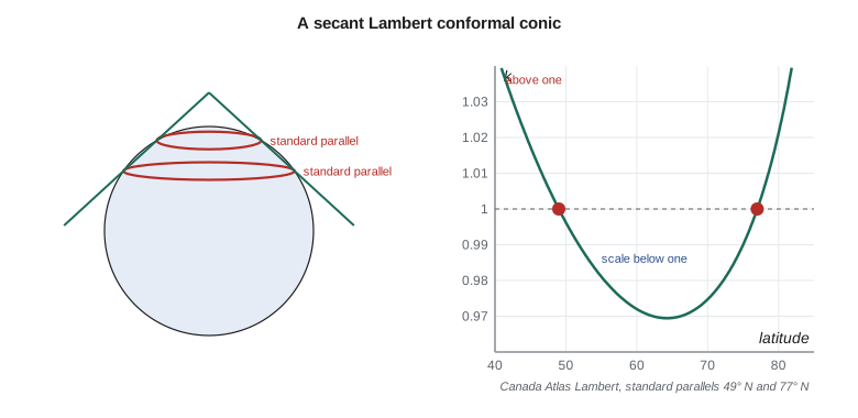
National mapping in Canada uses Lambert conformal conics with standard parallels at 49° N and 77° N, which span the country's latitude range. The Canada Atlas Lambert (EPSG:3978) with its central meridian at 95° W and the very similar Statistics Canada Lambert are used for national thematic and census maps, and Quebec, Ontario and other provinces use Lambert conics for provincial-scale mapping. Aeronautical charts in North America are Lambert conformal conics because straight lines on them are very nearly great circles and distances can be scaled from them with small error.
import math
a = 6378137.0; f = 1 / 298.257222101; e = math.sqrt(f * (2 - f))   # GRS80

def _m(p): return math.cos(p) / math.sqrt(1 - (e * math.sin(p)) ** 2)
def _t(p): return math.tan(math.pi / 4 - p / 2) / ((1 - e * math.sin(p)) / (1 + e * math.sin(p))) ** (e / 2)

class LCC:
    """Lambert conformal conic with two standard parallels (degrees, m)."""
    def __init__(self, lat1, lat2, lat0, lon0, fe=0.0, fn=0.0):
        p1, p2, p0 = map(math.radians, (lat1, lat2, lat0))
        self.n = (math.log(_m(p1)) - math.log(_m(p2))) / (math.log(_t(p1)) - math.log(_t(p2)))
        self.F = _m(p1) / (self.n * _t(p1) ** self.n)
        self.r0 = a * self.F * _t(p0) ** self.n
        self.lon0, self.fe, self.fn = lon0, fe, fn
    def forward(self, lat, lon):
        p = math.radians(lat); r = a * self.F * _t(p) ** self.n
        th = self.n * math.radians(lon - self.lon0)
        E = self.fe + r * math.sin(th); N = self.fn + self.r0 - r * math.cos(th)
        k = r * self.n / (a * _m(p))                  # point scale factor
        return E, N, k, math.degrees(th)               # th is the grid convergence
    def inverse(self, E, N):
        dx, dy = E - self.fe, self.r0 - (N - self.fn)
        r = math.copysign(math.hypot(dx, dy), self.n); th = math.atan2(dx, dy)
        t = (r / (a * self.F)) ** (1 / self.n); p = math.pi / 2 - 2 * math.atan(t)
        for _ in range(30):
            pn = math.pi / 2 - 2 * math.atan(t * ((1 - e * math.sin(p)) / (1 + e * math.sin(p))) ** (e / 2))
            if abs(pn - p) < 1e-15: break
            p = pn
        return math.degrees(p), self.lon0 + math.degrees(th / self.n)

# NAD83 / Canada Atlas Lambert (EPSG:3978): standard parallels 49 N and 77 N
atlas = LCC(49, 77, 49, -95)
lat, lon = 49.69673058, -112.82708789          # pillar CR1, Lethbridge
E, N, k, g = atlas.forward(lat, lon)
print(f"Canada Atlas Lambert: E = {E:12.3f}  N = {N:12.3f}  k = {k:.6f}  convergence = {g:.4f} deg")
print("inverse:", tuple(round(v, 9) for v in atlas.inverse(E, N)))

print("\nScale along a meridian of the Canada Atlas Lambert")
for L in (42, 49, 56, 63, 70, 77, 83):
    print(f"  latitude {L:2d}: k = {atlas.forward(L, -95)[2]:.4f}")

# A district projection: a cone cut through the district at 49.6 N and 49.8 N
dist = LCC(49.6, 49.8, 49.5, -112.8, 100000, 100000)
print("\nDistrict cone (standard parallels 49.6 and 49.8 N):")
for L in (49.5, 49.6, 49.7, 49.8, 49.9):
print(f" latitude {L:.1f}: k = {dist.forward(L, -112.8)[2]:.8f} ({(dist.forward(L, -112.8)[2]-1)*1e6:+.2f} ppm)")Canada Atlas Lambert: E = -1266022.956 N = 255971.473 k = 0.997359 convergence = -16.0585 deg inverse: (49.69673058, -112.82708789) Scale along a meridian of the Canada Atlas Lambert latitude 42: k = 1.0331 latitude 49: k = 1.0000 latitude 56: k = 0.9788 latitude 63: k = 0.9697 latitude 70: k = 0.9747 latitude 77: k = 1.0000 latitude 83: k = 1.0539 District cone (standard parallels 49.6 and 49.8 N): latitude 49.5: k = 1.00000455 (+4.55 ppm) latitude 49.6: k = 1.00000000 (+0.00 ppm) latitude 49.7: k = 0.99999848 (-1.52 ppm) latitude 49.8: k = 1.00000000 (+0.00 ppm) latitude 49.9: k = 1.00000456 (+4.56 ppm)
In the Canada Atlas Lambert, CR1 lies 1,266 km west and 256 km north of the origin at 49° N, 95° W. Its scale factor is 0.997359, 2,641 ppm too small, because the district lies just north of the southern standard parallel; and the grid convergence is −16.06°, a large angle because the district is nearly 18° of longitude west of the central meridian. Along the meridian the scale runs from 1.033 at 42° N through exactly 1 at 49° N and 77° N, to a minimum of about 0.970 near 63° N. These numbers are acceptable for a national atlas, where the distortion is far smaller than the width of a printed line at map scale, and unacceptable for any measurement. The narrow cone at the end of the code, with standard parallels at 49.6° and 49.8°, holds the scale within 5 ppm across the whole district. Its \(\rho\) and \(n\) are huge and close to those of a cylinder, as expected for a cone so close to a single parallel.
Choosing standard parallels
For a region spanning latitudes \(\varphi_S\) to \(\varphi_N\), a common rule of thumb places the standard parallels one-sixth of the range in from each edge. This approximately balances the negative distortion in the middle against the positive distortion at the edges, so that their largest values are about equal in size. For a band 4° wide, the parallels go 0.67° in from each edge and the largest scale error is roughly 340 ppm; for a band 1° wide, about 20 ppm. The error grows with the square of the band's width, as lesson 1 predicted. State plane designers in 1933 and 1983 chose zones and parallels so that the maximum scale error would generally not exceed 1 part in 10,000 (100 ppm), which needed zones about 250 km wide in latitude. Montana's single zone, adopted in 1983 to replace three older zones, accepts a larger error in exchange for one coordinate system statewide.
| Band width | Standard parallels in from edges | Largest scale error, approx. | Typical use |
|---|---|---|---|
| 0.2° (22 km) | 0.03° | 1 ppm | Project or low-distortion zone |
| 1° (111 km) | 0.17° | 20 ppm | County-scale zone |
| 2.5° (280 km) | 0.42° | 130 ppm | 1983 state plane zone |
| 4° (445 km) | 0.67° | 340 ppm | Large state zone |
| 28° (3,100 km) | chosen for the country | several thousand ppm | National atlas |
Standard parallels can also be replaced by a single standard parallel and a scale factor less than one on it, the one-standard-parallel form of the Lambert conic (EPSG method 'Lambert Conic Conformal (1SP)'). The two forms describe the same family: a 1SP zone with \(k_0 < 1\) is identical to a 2SP zone with two parallels either side of the central one. Software accepts both, and confusing them is a common source of wrong coordinates when a definition is typed in by hand.
The Albers equal-area conic
Heinrich Christian Albers described an equal-area conic in 1805. Its parallels are spaced so that the area between any two of them is correct, which keeps areas true everywhere. The scale along the parallels \(k\) and along the meridians \(h\) are reciprocals, \(hk = 1\), and \(k = 1\) on two standard parallels. Between them parallels are compressed and meridians stretched; outside them the opposite. For a region the size of a province or state, shape distortion is modest: angular distortion is no more than a degree or so. Albers is the standard projection for land-cover, agricultural and census statistics in North America: the US national land cover and cropland data are distributed in a conterminous-states Albers projection with standard parallels 29.5° N and 45.5° N, and British Columbia's provincial mapping uses an Albers projection with standard parallels at 50° N and 58.5° N. For the district's annual report of irrigated area by crop, Leah used an Albers projection centred on the district, so that the areas compared on the page would be correct.
Equidistant and other conics
The equidistant conic keeps true scale along all meridians and along its standard parallels; it is a compromise between the conformal and equal-area conics and appears in atlases of countries and continents. The polyconic projection, which uses a different cone for every parallel, was the projection of the US Geological Survey's topographic quadrangles until the mid-twentieth century and is encountered on old maps; it is neither conformal nor equal-area, but over a single quadrangle its distortion is negligible. Old cadastral and topographic data on polyconic coordinates should be reprojected with care, because many software packages implement it only approximately.
Worked problem
Convergence on a Lambert conic
On the Canada Atlas Lambert, the cone constant is \(n \approx 0.9008\). What is the grid convergence at CR1, longitude 112.827° W, with central meridian 95° W?
Show solution
- \[\gamma = n\,(\lambda - \lambda_0) = 0.9008 \times (-112.827 + 95.000)\]
- \[\gamma = 0.9008 \times (-17.827) = -16.06^\circ\]
Answer: True north at CR1 points about 16° east of grid north on this projection (grid north lies 16° west of true north); the code gives −16.0585°. Bearings scaled from a national atlas map are therefore wrong by about 16° unless corrected.
Worked problem
Standard parallels for a band
A Lambert zone is to cover southern Alberta from 49.0° N to 52.0° N. Where should the standard parallels go by the one-sixth rule?
Show solution
- \[\Delta = (52.0 - 49.0)/6 = 0.5^\circ\]
- \[\varphi_1 = 49.0 + 0.5 = 49.5^\circ, \qquad \varphi_2 = 52.0 - 0.5 = 51.5^\circ\]
Answer: Standard parallels at these latitudes give a largest scale error of about −150 ppm in the middle and +190 ppm at the edges, similar in size and opposite in sign.
Common mistakes
MistakeUsing a national atlas projection for measurements at a site.
InsteadIts scale and convergence at the site can be thousands of ppm and many degrees.
MistakeConfusing the 1SP and 2SP forms of the Lambert conic when entering parameters.
InsteadCheck which method the definition uses and that the parameters match it.
MistakeForgetting grid convergence when comparing bearings.
InsteadOn a conic, convergence is n(λ − λ0); apply it to convert grid to true bearings.
MistakeUsing a conformal conic for an area statistics map.
InsteadUse an equal-area conic such as Albers.
MistakeReprojecting old polyconic data without checking the software's implementation.
InsteadTest known points before converting a whole data set.
Summary and key terms
- Conic projections draw meridians as straight lines from an apex and parallels as circular arcs; the cone constant n sets the angle between meridians.
- The Lambert conformal conic is conformal; scale depends only on latitude and is one on the standard parallels.
- Lambert zones suit regions long east-west; distortion depends only on distance north or south of the standard band.
- Grid convergence on a conic is n(λ − λ0).
- The one-sixth rule balances distortion between the middle and the edges of a band.
- The Albers equal-area conic keeps area and is standard for statistics maps.
- Cone constant
- The ratio n of the angle between meridians on the map to their difference in longitude.
- Standard parallel
- A parallel along which the scale factor is exactly one.
- Lambert conformal conic
- The conformal conic projection, used for east-west zones and aeronautical charts.
- Albers equal-area conic
- The equal-area conic projection, standard for statistics maps.
- Grid convergence
- The angle between grid north and true north at a point.
- False origin
- The point given the false easting and northing to keep coordinates positive.
Practice problems
Work each problem on paper first, then reveal the answer to check.
What happens to a conic projection as the cone constant approaches zero?
Show answer
It becomes a cylindrical projection.
On a Lambert zone with two standard parallels, is the scale between them greater or less than one?
Show answer
Less than one.
Why does a Lambert zone's distortion not depend on longitude?
Show answer
Its scale is a function of latitude only, so isocols are parallels.
Which conic is used for national land-cover statistics, and why?
Show answer
Albers equal-area, because area comparisons must be correct.
By how much does the largest error of a Lambert band change if the band is made half as wide?
Show answer
It falls to about one quarter.
Lesson quiz · 5 questions
Score 60% or more to complete this lesson.
Create a free account to save your progress, take quizzes and earn a certificate.