
GEOM-340 · Lesson 3 of 12 · 23 min
Cylindrical projections
Cylindrical projections are the first family most people meet, because the most familiar world map, Mercator's, is one of them and because every web map that a district employee opens on a phone uses a variant of it. Theo Martel, who builds the district's web services, asked Leah why the coordinates in the district's tile cache did not match the coordinates in the GIS even though both were labelled 'Mercator'. This lesson answers that question and sets up the transverse Mercator projection of lesson 6, which is a cylindrical projection turned on its side.
The normal cylindrical family
In the normal aspect, the cylinder touches the globe along the equator, or cuts it along two parallels equally north and south of it. Every normal cylindrical projection has the same structure:
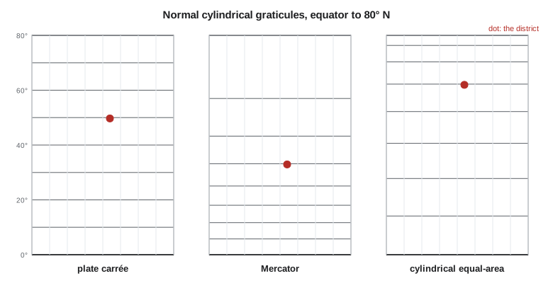
where \(\lambda_0\) is the central meridian, \(k_0\) the scale along the equator (or the standard parallels, for a secant form), and \(F(\varphi)\) a function of latitude alone that sets the spacing of the parallels. Meridians are equally spaced vertical lines and parallels are horizontal lines. On a sphere the scale along every parallel is \(k = k_0\sec\varphi\), whatever \(F\) is, because each parallel is stretched to the length of the equator. The choice of \(F\) fixes the scale along the meridian, \(h = F'(\varphi)\), and with it the projection's property: \(F = \varphi\) gives the plate carrée (equidistant along meridians), \(F = \sin\varphi\) the Lambert cylindrical equal-area, and \(F = \ln\tan(\pi/4 + \varphi/2)\) the Mercator, which is conformal because it makes \(h = k\) everywhere.
| Projection | Spacing function F(φ) | Property | Notes |
|---|---|---|---|
| Plate carrée | φ | Equidistant along meridians | Latitude and longitude plotted directly; common default for raw data |
| Equirectangular | φ, with k₀ = cos φ₁ | Equidistant along meridians | True scale along two chosen parallels |
| Mercator | ln tan(π/4 + φ/2) | Conformal | Rhumb lines straight; poles at infinity |
| Lambert cylindrical equal-area | sin φ | Equal-area | Variants (Behrmann, Gall-Peters) change the standard parallels |
| Miller cylindrical | 1.25 ln tan(π/4 + 0.4φ) | Compromise | A softened Mercator for world maps |
Mercator's projection
Gerardus Mercator published his world map in 1569 for navigators. Its purpose was a property that only a conformal cylindrical projection has: a line of constant compass bearing, a rhumb line or loxodrome, plots as a straight line. A navigator could draw a straight line from port to destination, measure its angle from a meridian with a protractor and steer that course. Mercator built the spacing of his parallels by construction; the exact formula, the integral of \(\sec\varphi\), was found later in the seventeenth century, when it was noticed that tables of the spacing matched tables of logarithmic tangents. On a sphere
The scale grows without limit toward the poles, which cannot be shown. At 60° the scale is 2, so areas are enlarged four times; at 80°, nearly 6, so areas are enlarged 33 times. This is why Greenland looks as large as Africa on a Mercator world map although Africa is about fourteen times larger. For a navigational chart or a map of a narrow band near the equator, Mercator is excellent; for a world map meant to show the relative size of countries, it is a poor choice.
On the ellipsoid, latitude is replaced by the isometric latitude \(\psi\), which plays the same role for an ellipsoid as \(\ln\tan(\pi/4 + \varphi/2)\) does for a sphere:
with \(a\) the semi-major axis and \(e\) the eccentricity. The inverse cannot be written in closed form and is solved by a short iteration, as in the code below. Isometric latitude appears again in the Lambert conformal conic and transverse Mercator projections; it is the quantity that makes a conformal projection of an ellipsoid possible.
Web Mercator
Most online maps and tile services use a projection registered as EPSG:3857, commonly called Web Mercator or Pseudo-Mercator. It takes latitude and longitude on the WGS 84 ellipsoid and puts them through the spherical Mercator formula, using the ellipsoid's semi-major axis as the sphere's radius. This was a practical decision by the companies that built the first web maps: the spherical formula is simpler and faster, the world fits a square, and square tiles divide neatly at each zoom level. The result is not quite conformal, because ellipsoidal latitudes are used with spherical formulas; the error is small, a difference of about 0.3 % between the north-south and east-west scales at middle latitudes (up to about 0.7 % near the equator), and invisible on a screen.
The northings, however, differ substantially from those of a true ellipsoidal Mercator. Treating EPSG:3857 coordinates as if they were ellipsoidal Mercator, or the reverse, shifts features north or south by tens of kilometres. Web Mercator also inherits all of Mercator's area and distance distortion, so measurements made directly on its coordinates are wrong by the factor \(\sec\varphi\). Well-behaved web mapping software stores data in another CRS, reprojects to EPSG:3857 only for display, and computes distances and areas on the ellipsoid. GEOM-330 used EPSG:3857 only to cut tiles; nothing should be measured in it.
import math
a = 6378137.0; f = 1 / 298.257222101; e = math.sqrt(f * (2 - f))   # GRS80

def merc_forward(lat, lon, lon0=0.0, k0=1.0):
    """Ellipsoidal Mercator: degrees -> m, plus the point scale factor."""
    p = math.radians(lat)
    psi = math.atanh(math.sin(p)) - e * math.atanh(e * math.sin(p))   # isometric latitude
    x = k0 * a * math.radians(lon - lon0); y = k0 * a * psi
    k = k0 * math.sqrt(1 - (e * math.sin(p)) ** 2) / math.cos(p)
    return x, y, k

def merc_inverse(x, y, lon0=0.0, k0=1.0):
    psi = y / (k0 * a); p = math.atan(math.sinh(psi))
    for _ in range(20):                        # iterate for geodetic latitude
        p_new = math.asin(math.tanh(psi + e * math.atanh(e * math.sin(p))))
        if abs(p_new - p) < 1e-15: break
        p = p_new
    return math.degrees(p), lon0 + math.degrees(x / (k0 * a))

def web_mercator(lat, lon):
    """EPSG:3857: ellipsoidal latitude and longitude put through the spherical formula."""
    return a * math.radians(lon), a * math.log(math.tan(math.pi / 4 + math.radians(lat) / 2))

lat, lon = 49.69673058, -112.82708789          # pillar CR1
x, y, k = merc_forward(lat, lon)
xw, yw = web_mercator(lat, lon)
print(f"CR1 ellipsoidal Mercator  x = {x:14.3f}  y = {y:14.3f}  k = {k:.6f}")
print(f"CR1 web Mercator (3857)   x = {xw:14.3f}  y = {yw:14.3f}")
print(f"northing difference web - ellipsoidal = {yw - y:,.1f} m")
la, lo = merc_inverse(x, y)
print(f"inverse check: {la:.9f}, {lo:.9f}  (round trip error {abs(la-lat)*111e3*1000:.4f} mm)")

# A rhumb line is a straight line on a Mercator map
def rhumb(lat1, lon1, lat2, lon2):
    x1, y1, _ = merc_forward(lat1, lon1); x2, y2, _ = merc_forward(lat2, lon2)
    az = math.degrees(math.atan2(x2 - x1, y2 - y1)) % 360        # constant course
    # length along the rhumb line: meridian arc length divided by cos(course)
    def marc(phi):                        # meridian arc from the equator (series, mm-level)
        n = f / (2 - f); p = math.radians(phi)
        A = a / (1 + n) * (1 + n*n/4 + n**4/64)
        return A * (p - (3*n/2 - 9*n**3/16) * math.sin(2*p) + (15*n*n/16) * math.sin(4*p) - (35*n**3/48) * math.sin(6*p))
    dist = (marc(lat2) - marc(lat1)) / math.cos(math.radians(az))
    return az, dist

az, d = rhumb(lat, lon, 47.50600422, -111.29779092)            # CR1 Lethbridge -> CR1 Great Falls
print(f"rhumb line Lethbridge -> Great Falls: course {az:.4f} deg, length {d/1000:.3f} km")
for L in (0, 30, 49.7, 60, 80):
print(f"Mercator scale at latitude {L:4.1f}: k = {merc_forward(L, 0)[2]:.4f}")CR1 ellipsoidal Mercator x = -12559853.972 y = 6361314.688 k = 1.542981 CR1 web Mercator (3857) x = -12559853.972 y = 6393919.634 northing difference web - ellipsoidal = 32,604.9 m inverse check: 49.696730580, -112.827087890 (round trip error 0.0000 mm) rhumb line Lethbridge -> Great Falls: course 155.1609 deg, length 268.447 km Mercator scale at latitude 0.0: k = 1.0000 Mercator scale at latitude 30.0: k = 1.1537 Mercator scale at latitude 49.7: k = 1.5431 Mercator scale at latitude 60.0: k = 1.9950 Mercator scale at latitude 80.0: k = 5.7400
For pillar CR1 at Lethbridge, the ellipsoidal Mercator northing is 6,361,314.688 m and the Web Mercator northing 6,393,919.634 m: the same point, 32.6 km apart in the two systems. The eastings agree because both use the same formula along the equator. The point scale factor at CR1 is 1.5430, so a 1 km line at the district is drawn 1.543 km long, and the inverse returns the original latitude and longitude to well under a millimetre. A rhumb line from Lethbridge to Great Falls has a constant course of 155.16° and a length of 268.45 km, slightly longer than the geodesic between the same points, which crosses the meridians at changing angles. Over this distance the difference is a few hundred metres, which matters to a pilot planning fuel and not at all to a surveyor, who never uses rhumb lines.
Equal-area and compromise cylinders
The Lambert cylindrical equal-area projection, published by Johann Heinrich Lambert in 1772, keeps areas correct by compressing the parallels toward the poles exactly as fast as the parallels are stretched. With the cylinder tangent at the equator, shapes near the poles are flattened beyond recognition. Making it secant at a standard parallel \(\varphi_1\), with \(x = R\cos\varphi_1(\lambda - \lambda_0)\) and \(y = R\sin\varphi/\cos\varphi_1\), moves the undistorted parallels north and south. The Behrmann (standard parallels 30°) and Gall-Peters (45°) versions are examples. They are used for world maps of quantities per unit area, such as population density or crop area, where the reader's eye judges amounts by area. A district-scale equal-area map is usually drawn instead with an equal-area conic or azimuthal projection, which have far less shape distortion over a small region, as lessons 4 and 5 show.
Compromise cylinders, such as Miller's of 1942, reduce Mercator's polar exaggeration by scaling the latitude before applying the Mercator formula. They are neither conformal nor equal-area and are used only for general world maps. The plate carrée deserves a separate warning: although no cartographer would choose it, it is what a GIS draws by default when data in latitude and longitude are displayed without a projection, so it is the most commonly seen projection in the world and the source of many distorted maps of northern regions.
Transverse and oblique cylinders
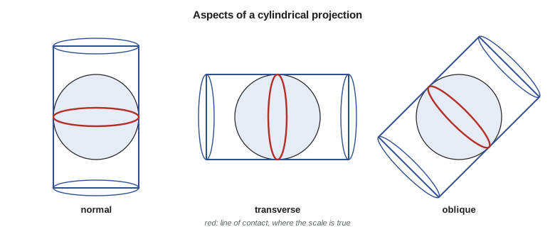
Turning the cylinder through 90° so that it touches a meridian gives the transverse aspect. The transverse form of the plate carrée is the Cassini (or Cassini-Soldner) projection, equidistant along the central meridian and along lines at right angles to it. It was used in the eighteenth and nineteenth centuries for topographic and cadastral surveys of narrow regions, including many European national surveys, and old cadastral records in some places are still on Cassini coordinates. It is not conformal; its scale error grows with the square of the distance from the central meridian in the east-west direction only, so it suits areas only a few tens of kilometres wide.
The transverse form of the Mercator is conformal and is the basis of UTM, of most provincial and state systems in long north-south regions and of many national grids; lesson 6 treats it in detail. Turning the cylinder to an arbitrary angle gives the oblique Mercator, which touches the globe along a great circle that can follow a region running diagonally. The Hotine oblique Mercator is used for Alaska's southeastern panhandle in the state plane system, for national grids such as those of Switzerland and Malaysia, and for several low-distortion projections along diagonal corridors such as highways and pipelines. For a canal or pipeline running at 45° to the meridians, an oblique Mercator can hold distortion to a few parts per million along its whole length.
Worked problem
Mercator scale and area at the district
On a Mercator world map with \(k_0 = 1\), what is the scale at Lethbridge, latitude 49.70°, and how much is the area of a 1 km² field enlarged? Use the sphere.
Show solution
- \[k = \sec 49.70^\circ = \frac{1}{0.64679} = 1.5461\]
- \[s = k^2 = 1.5461^2 = 2.390\]
Answer: The field is drawn 2.39 times its true area. The ellipsoidal formula gives 1.5430 at CR1, slightly less because the ellipsoid's parallels are a little longer than the sphere's at this latitude.
Worked problem
Choosing the standard parallels of an equidistant cylinder
A display of the district in latitude and longitude is to be corrected so that east-west and north-south distances are true at the district's centre, latitude \(\varphi_1\). What should the east-west scale \(k_0\) be?
Show solution
- \[x = R\cos\varphi_1\,(\lambda - \lambda_0), \qquad y = R\,\varphi\]
- \[k = \frac{\cos\varphi_1}{\cos\varphi} = 1 \text{ when } \varphi = \varphi_1\]
Answer: Set \(k_0 = \cos\varphi_1\): the equirectangular projection with standard parallel \(\varphi_1\). Over the district the remaining error is a few hundred ppm north and south of the standard parallel, adequate for a quick display but not for measurement.
Common mistakes
MistakeMeasuring distances or areas in Web Mercator coordinates.
InsteadUse EPSG:3857 only for display; measure on the ellipsoid or in a suitable projected CRS.
MistakeTreating EPSG:3857 and an ellipsoidal Mercator as interchangeable.
InsteadTheir northings differ by tens of kilometres at middle latitudes.
MistakeUsing a Mercator world map to compare the sizes of countries.
InsteadUse an equal-area projection for area comparisons.
MistakeDisplaying unprojected latitude and longitude for northern regions.
InsteadChoose a projection; the plate carrée stretches east-west distances by sec φ.
MistakeApplying a Cassini projection's coordinates as if they were conformal.
InsteadCassini is equidistant along its central meridian only; check old cadastral systems carefully.
Summary and key terms
- Normal cylindrical projections draw meridians and parallels as straight lines at right angles; the parallel spacing F(φ) sets the property.
- Mercator (1569) is the conformal cylinder; rhumb lines are straight and scale grows as sec φ.
- On the ellipsoid, Mercator uses the isometric latitude; its inverse is iterative.
- Web Mercator (EPSG:3857) applies spherical formulas to ellipsoidal coordinates; it is for display only.
- Lambert's cylindrical equal-area and its secant variants keep area at the expense of shape.
- Transverse cylinders give Cassini and transverse Mercator; oblique Mercator follows diagonal regions.
- Rhumb line
- A line of constant bearing, straight on a Mercator map.
- Isometric latitude
- A function of latitude that makes conformal mapping of the ellipsoid possible.
- Web Mercator
- EPSG:3857, the spherical Mercator formula applied to WGS 84 coordinates for web tiles.
- Plate carrée
- The projection that plots longitude and latitude directly as x and y.
- Cassini projection
- The transverse equidistant cylinder, once used for narrow survey regions.
- Oblique Mercator
- A conformal cylinder touching the globe along an inclined great circle.
Practice problems
Work each problem on paper first, then reveal the answer to check.
What is the Mercator area scale at latitude 60°?
Show answer
sec² 60° = 4.
Why are rhumb lines straight on a Mercator map?
Show answer
The projection is conformal and its meridians are parallel, so a constant angle with the meridians is a straight line.
Which spacing function gives an equal-area cylinder?
Show answer
F(φ) = sin φ.
A service publishes tiles in EPSG:3857. May a buffer of 100 units be drawn in those coordinates?
Show answer
Only approximately; the units are not true metres at the district's latitude.
Which cylindrical aspect suits a pipeline running north-east?
Show answer
Oblique Mercator, with its line of contact along the pipeline.
Lesson quiz · 5 questions
Score 60% or more to complete this lesson.
Create a free account to save your progress, take quizzes and earn a certificate.