
GEOM-230 · Lesson 7 of 12 · 20 min
Height systems
The irrigation district wants to extend its main canal from Coulee Ridge toward the foothills, and the design depends on heights along a 25 km line that climbs about 550 m. Leah Tran added up the levelled height differences on the line and was surprised when Ruth Albrecht told her that the sum was not the orthometric height difference between the two ends: it was almost a decimetre short. The canal itself does not care about any particular height system. Water flows from higher to lower potential, and a canal is level when its water surface lies on one level surface. But the numbers written on the drawings must come from some definition of height, and there are several. This lesson explains why levelling alone is not enough, what geopotential numbers are, and how dynamic, orthometric and normal heights are defined from them.
Why levelling depends on the route
Spirit levelling measures the vertical separation between the local level surfaces through two staff positions, set after set. Lesson 5 showed that level surfaces are not parallel: they converge where gravity is stronger, toward the poles and over dense rock. Suppose two benchmarks lie on the same level surface, so that water would not flow between them. Levelling north from one along a route at low elevation and back along a route over a ridge would cross the level surfaces at places where they are differently spaced. The sum of the measured differences around the loop would not be zero, even with perfect instruments. This is the theoretical loop misclosure, and over long lines in mountainous country it reaches several centimetres.
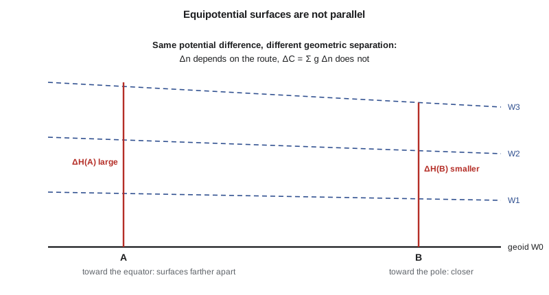
The cure is to weight each measured difference by gravity. The work done against gravity in lifting a unit mass through a levelled difference \(dn\) is \(g\,dn\). Summed around any closed loop, the work is zero, because gravity is a conservative field:
This is why Ruth wanted gravity at the benchmarks. With gravity, levelled differences become potential differences, which are route-independent and form the foundation of every rigorous height system.
Geopotential numbers
The geopotential number of a point P is the difference between the potential of the geoid and the potential at P:
It is positive above the geoid and increases with height. Its unit is the square metre per second squared; the older geopotential unit, 1 gpu = 10 m²/s², makes the numerical value of \(C\) in gpu close to the height in metres, because gravity is close to 10 m/s². Geopotential numbers are the natural heights of physics: all points on a level surface share the same \(C\), and water flows from larger to smaller \(C\). Their drawback is that they are not lengths. Engineers and the public want metres, so each height system divides \(C\) by a gravity value of some kind. The choice of that gravity value distinguishes the systems.
Dynamic heights
The simplest choice is a constant: normal gravity at latitude 45°, \(\gamma_{45} = 9.806\,199\) m/s² on GRS80. The dynamic height is
Points on the same level surface have exactly the same dynamic height, which makes dynamic heights ideal where the main question is whether water will flow. The International Great Lakes Datum, used by Canada and the United States to manage the lakes and the St. Lawrence system, is expressed in dynamic heights for that reason. The drawback is that a dynamic height is not the geometric distance above anything. Wherever mean gravity along the plumb line differs from \(\gamma_{45}\), dynamic heights differ from orthometric heights: a difference of 20 mGal, two thousandths of a per cent, changes a 1000 m height by 20 mm, and the differences grow with latitude and height. Levelled differences therefore need dynamic corrections, which can be large on long lines far from 45°.
Orthometric heights
The orthometric height is the geometric length of the plumb line from the geoid to the point. It follows from the geopotential number by dividing by the mean value of gravity along the plumb line inside the Earth:
Gravity inside the topography cannot be measured, so \(\bar g\) must be estimated from surface gravity and a model of the rock density. The Helmert approximation assumes a uniform Bouguer slab of density 2670 kg/m³ and a normal free-air gradient, which gives a mean gravity halfway down the plumb line of
that is, surface gravity plus 0.0424 mGal for every metre of height. Because \(H\) appears on both sides, the computation iterates, but it converges in two or three steps. Helmert orthometric heights are the official heights of both CGVD2013 and NAVD 88. More refined orthometric heights model the actual density and terrain, and they differ from Helmert heights by a few centimetres in high mountains.
Orthometric heights have a clear geometric meaning, and they combine directly with GNSS through \(h = H + N\). Their drawback is that points on the same level surface do not, in general, have the same orthometric height, because the level surfaces are not parallel. Two points on one lake can differ in orthometric height by centimetres.
Normal heights
Mikhail Molodensky avoided the unknown gravity inside the Earth by dividing instead by normal gravity, which can be computed exactly. The normal height is
where \(\bar\gamma\) is the mean normal gravity along the normal plumb line between the ellipsoid and the height \(H^{*}\) above it. Normal heights refer not to the geoid but to a closely related surface, the quasigeoid, and the separation between the quasigeoid and the ellipsoid is the height anomaly \(\zeta\), so that \(h = H^{*} + \zeta\). Over the oceans the quasigeoid and geoid coincide; on land they differ by roughly \(\Delta g_B H/\gamma\), where \(\Delta g_B\) is the Bouguer anomaly. On the prairies the difference is about a decimetre at 1500 m; in high mountains it can exceed a metre. Most European countries use normal heights.
Worked problem
Geopotential number and dynamic height of BM A
Benchmark A has a published orthometric height of 902.418 m and measured surface gravity \(g = 9.807\,865\) m/s². Find its geopotential number with Helmert's mean gravity, and its dynamic height.
Show solution
- \[\bar g = 9.807\,865 + 0.0424 \times 10^{-5} \times 902.418 = 9.808\,247\,6\ \text{m/s}^2\]
- \[C = H\,\bar g = 902.418 \times 9.808\,247\,6 = 8851.139\ \text{m}^2/\text{s}^2 = 885.1139\ \text{gpu}\]
- \[H^{\text{dyn}} = \frac{C}{\gamma_{45}} = \frac{8851.139}{9.806\,199} = 902.607\ \text{m}\]
- \[H^{\text{dyn}} - H = 902.607 - 902.418 = +0.189\ \text{m}\]
Answer: The geopotential number of BM A is 8851.139 m²/s², and its dynamic height is 902.607 m, 189 mm larger than its orthometric height because gravity at the benchmark is stronger than normal gravity at 45°.
Heights along the canal line
The program below carries a geopotential number along the canal line from BM A, using the levelled differences and the mean of the gravity values at the two ends of each section. At each benchmark it computes the Helmert orthometric height, the normal height and the dynamic height, and compares them with the raw sum of the levelled differences.
# Geopotential numbers and four kinds of height along a line of spirit levels
import math

a, f = 6378137.0, 1 / 298.257222101
ge, k, e2 = 9.7803267715, 0.001931851353, f * (2 - f)
def gamma0(lat):
    s2 = math.sin(math.radians(lat)) ** 2
    return ge * (1 + k * s2) / math.sqrt(1 - e2 * s2)
gamma45 = gamma0(45.0)

# Benchmarks westward from BM A towards the foothills: latitude, measured gravity (m/s^2),
# and the measured height difference from the previous benchmark (m)
line = [("BM A", 49.7088, 9.807865, None),
        ("K1", 49.6510, 9.807625, 95.312),
        ("K2", 49.5893, 9.807155, 211.744),
        ("K3", 49.5214, 9.806615, 240.128)]
H_A = 902.418                                       # published orthometric height of BM A

# Helmert: mean gravity along the plumb line = surface g + 0.0424 mGal per m of height
def gbar_helmert(g, H): return g + 0.0424e-5 * H                # half the 0.0848 mGal/m Poincare-Prey gradient
C = H_A * gbar_helmert(line[0][2], H_A)                         # geopotential number of BM A
raw = H_A
rows = []
for i, (name, lat, g, dn) in enumerate(line):
    if dn is not None:
        g_prev = line[i - 1][2]
        C += dn * (g + g_prev) / 2                   # dC = mean gravity along the section times dn
        raw += dn
    # Helmert orthometric height: solve H = C / (g + 0.0424 mGal/m * H) by iteration
    H = C / g
    for _ in range(5):
        H = C / gbar_helmert(g, H)
    # Normal height: C divided by mean normal gravity along the normal plumb line
    Hn = C / gamma0(lat)
    for _ in range(5):
        Hn = C / (gamma0(lat) * (1 - (1 + f + 0.003449786 - 2 * f * math.sin(math.radians(lat)) ** 2) * Hn / a + Hn * Hn / (a * a)))
    Hdyn = C / gamma45
    rows.append((name, C, raw, H, Hn, Hdyn))

print("name   C (m^2/s^2)   sum of dn    Helmert H    normal H*    dynamic")
for name, C, raw, H, Hn, Hdyn in rows:
    print(name.ljust(5), format(C, "12.3f"), format(raw, "11.4f"), format(H, "12.4f"), format(Hn, "12.4f"), format(Hdyn, "11.4f"))
name, C, raw, H, Hn, Hdyn = rows[-1]
print()
print("at", name, ": orthometric correction (H - sum dn) =", format(1000 * (H - raw), "+.1f"), "mm")
print("normal minus orthometric =", format(1000 * (Hn - H), "+.1f"), "mm;  dynamic minus orthometric =", format(1000 * (Hdyn - H), "+.1f"), "mm")
print("geopotential numbers in geopotential units (1 gpu = 10 m^2/s^2):", round(C / 10, 4))name C (m^2/s^2) sum of dn Helmert H normal H* dynamic BM A 8851.139 902.4180 902.4180 902.3440 902.6065 K1 9785.935 997.7300 997.7454 997.6635 997.9335 K2 11862.591 1209.4740 1209.5221 1209.4230 1209.7032 K3 14217.499 1449.6020 1449.6957 1449.5759 1449.8480 at K3 : orthometric correction (H - sum dn) = +93.7 mm normal minus orthometric = -119.8 mm; dynamic minus orthometric = +152.3 mm geopotential numbers in geopotential units (1 gpu = 10 m^2/s^2): 1421.7499
At K3, 547 m above BM A, the raw sum of the levelled differences gives 1449.602 m, but the Helmert orthometric height is 1449.696 m. The 94 mm difference is the orthometric correction for this line. It arises because the line climbs into an area where gravity is about 125 mGal weaker, so the level surfaces are farther apart there than at BM A. The normal height at K3 is 120 mm below the orthometric height, reflecting the negative Bouguer anomaly of the region, and the dynamic height is 152 mm above it, because gravity at this latitude exceeds the 45° value. For the canal, the differences matter: a 94 mm error in the head at the upper end would change the design gradient noticeably.
The orthometric correction
In practice, national levelling networks are adjusted in geopotential numbers, and the heights are published in one system. A surveyor who levels a short line between published benchmarks applies an orthometric correction to the observed differences so that they agree with published orthometric heights. For a section from A to B it can be written
with \(\gamma_0\) an arbitrary constant, usually \(\gamma_{45}\). On flat ground the correction is negligible; on lines that climb hundreds of metres it reaches centimetres, as the program shows. For small sites with modest relief, such as the Coulee Ridge subdivision, it is a fraction of a millimetre and can be ignored.
| Height | Definition | Reference surface | Where used |
|---|---|---|---|
| Geopotential number C | W0 − W | Geoid | Network adjustment |
| Dynamic H dyn | C / γ45 | Geoid | Great Lakes (IGLD) |
| Orthometric H | C / mean g on plumb line | Geoid | CGVD2013, NAVD 88 |
| Normal H* | C / mean normal gravity | Quasigeoid | Most of Europe |
| Ellipsoidal h | Distance along the normal | Ellipsoid | GNSS; not physical |
Ellipsoidal heights complete the picture. They are purely geometric, come directly from GNSS, and have nothing to do with the flow of water. Two points with the same ellipsoidal height can differ in orthometric height by a metre if the geoid slopes between them. They are converted to physical heights through a geoid or quasigeoid model.
Common mistakes
MistakeSumming levelled differences over a long mountain line and calling the result an orthometric height difference.
InsteadApply the orthometric correction or work in geopotential numbers.
MistakeExpecting points on one lake to have equal orthometric heights.
InsteadOnly dynamic heights (and geopotential numbers) are equal on a level surface.
MistakeUsing surface gravity as the mean gravity along the plumb line.
InsteadAdd 0.0424 mGal per metre of height (Helmert) or use a density model.
MistakeMixing normal and orthometric heights.
InsteadThey refer to different surfaces and can differ by decimetres in high terrain.
MistakeTreating ellipsoidal heights as indicating water flow.
InsteadConvert to physical heights with a geoid model first.
Summary and key terms
- Levelled differences depend on the route because level surfaces are not parallel.
- Weighting by gravity gives route-independent geopotential numbers C = W0 − W.
- Dynamic heights divide C by γ45 and are equal on a level surface.
- Orthometric heights divide C by the mean gravity along the plumb line; Helmert's approximation adds 0.0424 mGal per metre.
- Normal heights divide C by mean normal gravity and refer to the quasigeoid.
- The orthometric correction reconciles raw levelling with published orthometric heights.
- CGVD2013 and NAVD 88 use Helmert orthometric heights; the Great Lakes use dynamic heights.
- Geopotential number
- The potential difference C = W0 − W between the geoid and a point.
- Dynamic height
- The geopotential number divided by normal gravity at 45° latitude.
- Orthometric height
- The length of the plumb line from the geoid to a point, equal to C divided by the mean gravity along it.
- Normal height
- The geopotential number divided by mean normal gravity; referred to the quasigeoid.
- Quasigeoid
- The reference surface for normal heights, close to the geoid.
- Orthometric correction
- The correction applied to levelled differences to obtain orthometric height differences.
Practice problems
Work each problem on paper first, then reveal the answer to check.
A point has C = 9 800.000 m²/s². What is its dynamic height?
Show answer
9800 / 9.806 199 = 999.368 m.
Surface gravity is 9.807 000 m/s² at H ≈ 1000 m. What is Helmert's mean gravity?
Show answer
9.807 000 + 0.0424e-5 × 1000 = 9.807 424 m/s².
With that mean gravity and C = 9 807.400 m²/s², what is the orthometric height?
Show answer
9807.400 / 9.807 424 ≈ 999.998 m.
Why is the orthometric correction negligible on the Coulee Ridge subdivision?
Show answer
Relief and distances are small, so gravity changes very little along the lines.
Which height system makes points on one level surface equal?
Show answer
Dynamic heights, or geopotential numbers.
Lesson quiz · 5 questions
Score 60% or more to complete this lesson.
Create a free account to save your progress, take quizzes and earn a certificate.