The geoid

When Grant Okonkwo's crew occupied benchmark A at Coulee Ridge with a GNSS receiver, the ellipsoidal height came out at 886.210 m. The published CGVD2013 height of the same mark is 902.418 m. The 16 m difference was not an error. It is the separation between the ellipsoid, to which GNSS heights refer, and the geoid, to which heights above sea level refer. Near Lethbridge the geoid lies about 16 m below the GRS80 ellipsoid. Knowing that separation to a centimetre or two at every point is what allows GNSS to deliver usable heights without running a level line from the nearest benchmark, and it is the reason Canada was able to redefine its vertical datum on the geoid in 2013.

What the geoid is

The geoid is the level surface of the Earth's gravity field that best coincides with mean sea level over the oceans. If the oceans were at rest, with no winds, currents, tides or differences in temperature and salinity, their surface would follow one level surface, and that surface, imagined as continuing under the continents, would be the geoid. Because it is a level surface, the geoid is everywhere perpendicular to the direction of gravity, and water does not flow along it. It is the natural zero for heights that tell which way water will flow.

The real sea surface departs from any level surface by up to one or two metres because of ocean currents, winds and density differences. This departure is called sea surface topography. For that reason, modern definitions do not tie the geoid to a particular tide gauge. Instead, the geoid is defined by a chosen value \(W_0\) of the gravity potential. In 2015 the International Association of Geodesy adopted a conventional global value of \(W_0 = 62\,636\,853.4\ \text{m}^2/\text{s}^2\). Canada and the United States had earlier agreed on \(W_0 = 62\,636\,856.0\ \text{m}^2/\text{s}^2\) for North America, which places the North American geoid about 26 cm below the global conventional one; the two countries chose their value to fit mean sea level around the continent's coasts.

Undulations

The height of the geoid above the reference ellipsoid is the geoid height or geoid undulation \(N\). Globally it ranges from about −106 m in the Indian Ocean south of India to about +85 m near New Guinea. These broad features reflect density differences deep in the mantle. Over North America the geoid lies below the GRS80 ellipsoid almost everywhere, with a broad low centred on Hudson Bay that is linked to the crust still rebounding after the last ice age. Shorter-wavelength features, of a few metres over tens of kilometres, follow topography and crustal density: mountains, sedimentary basins and buried intrusions.

Near the site the geoid height is about −16 m and changes smoothly, by a centimetre or two per kilometre. That slope is not negligible: over a 38 km pipeline the geoid changes by about half a metre, so a GNSS-derived height difference without a geoid correction would be wrong by that amount.

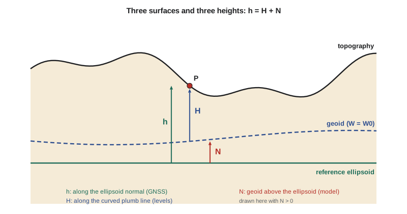
Ellipsoidal height, orthometric height and geoid height

An ellipsoidal height \(h\) is measured along the ellipsoid normal; an orthometric height \(H\) is measured along the curved plumb line from the geoid; the geoid height \(N\) is measured along the normal from the ellipsoid to the geoid. To a very good approximation,

The relation is not exact, because the plumb line is curved and is tilted from the normal by the deflection of the vertical, but the error is far below a millimetre for all practical situations. With \(N\) from a model, GNSS heights convert to orthometric heights by \(H = h - N\). For differences between two points,

and here the geoid model's relative accuracy matters more than its absolute accuracy. A model that is in error by 3 cm everywhere introduces no error at all in height differences; one whose error varies by 3 cm across the project does.

Disturbing potential and Bruns's formula

The difference between the actual potential \(W\) and the normal potential \(U\) of the level ellipsoid at the same point is the disturbing potential \(T = W - U\). It is small, of order a few hundred square metres per second squared, and it contains all the information about the irregularities of the field. On the geoid, where \(W = W_0\), and with the level ellipsoid having potential \(U_0 = W_0\), Bruns's formula links the geoid height to the disturbing potential:

Every geoid model rests on this formula. The task of physical geodesy is to determine \(T\) from gravity measurements. Stokes showed in 1849 that if gravity anomalies were known over the whole Earth, \(T\) and therefore \(N\) could be computed by an integral of the anomalies weighted by a function of the distance from the computation point. Nearby anomalies influence the result most, but distant ones are not negligible, so global data are needed.

How a geoid model is built

Modern geoid models combine three kinds of information, each covering a band of wavelengths. Satellite gravity from GRACE and GOCE, combined into a global geopotential model expressed as spherical harmonic coefficients, supplies the long wavelengths, from thousands of kilometres down to about 100 km. Terrestrial and airborne gravity measurements supply the medium wavelengths, down to a few kilometres. Digital elevation models supply the shortest wavelengths, through the gravitational effect of the terrain. In the common remove–compute–restore approach, the global model and the terrain effect are removed from the observed anomalies, the residual anomalies are integrated with a modified Stokes function, and the global model and terrain contributions are restored.

The result is a gravimetric geoid, which depends only on gravity and the adopted \(W_0\). Its accuracy in well-surveyed flat areas such as the prairies is a few centimetres; in mountains, where gravity data are sparse and the terrain is rough, errors can reach a decimetre or more. A hybrid geoid is a gravimetric geoid warped to fit the differences \(h - H\) at benchmarks with both GNSS and levelled heights. It reproduces a levelling-based datum, with all of that datum's errors, rather than the true geoid. GEOID18 in the United States is a hybrid model tied to NAVD 88; CGG2013a in Canada is a gravimetric model that defines CGVD2013 directly.

Geoid models are distributed as grids of \(N\) values at regular spacing in latitude and longitude, typically 1′ or 2′. Software interpolates in the grid, usually bilinearly or with a biquadratic or spline method. Bilinear interpolation is adequate when the grid is fine relative to the geoid's curvature.

Checking on benchmarks

A careful surveyor never trusts a GNSS-derived height until it has been compared with benchmarks of known height in the same project. The program below interpolates the geoid at CR1 and at two benchmarks, computes their heights from GNSS, and compares the benchmarks with their published values. The mean difference shows any bias between the GNSS heights, the geoid model and the vertical datum as realized locally; the spread shows whether a single offset is enough.

# Heights from GNSS: h = H + N with a geoid grid, checked on benchmarks
import math

# Geoid heights N (m) at grid nodes extracted from the national model around the site
lat0, lon0, step = 49.65, -112.90, 0.05          # south-west node and spacing, degrees
GRID = [[-16.203, -16.144, -16.087],             # row 0 at lat 49.65, columns at lon -112.90, -112.85, -112.80
        [-16.266, -16.207, -16.150],             # row 1 at lat 49.70
        [-16.329, -16.270, -16.211]]             # row 2 at lat 49.75

def geoid(lat, lon):
    x, y = (lon - lon0) / step, (lat - lat0) / step
    i, j = int(y), int(x); dy, dx = y - i, x - j
    n00, n01, n10, n11 = GRID[i][j], GRID[i][j + 1], GRID[i + 1][j], GRID[i + 1][j + 1]
    return (n00 * (1 - dx) * (1 - dy) + n01 * dx * (1 - dy) + n10 * (1 - dx) * dy + n11 * dx * dy)

def dms(d, m, s): return math.copysign(abs(d) + m / 60 + s / 3600, d)

points = {  # name: (lat, lon, ellipsoidal height h from GNSS, published orthometric height or None)
    "CR1": (dms(49, 41, 48.2301), -dms(112, 49, 37.5164), 893.412, None),
    "BM A": (dms(49, 42, 31.80), -dms(112, 51, 3.40), 886.210, 902.418),
    "BM B": (dms(49, 43, 40.10), -dms(112, 48, 20.25), 899.010, 915.207),
}
offsets = []
for name, (lat, lon, h, Hpub) in points.items():
    N = geoid(lat, lon)
    H = h - N
    line = name.ljust(5) + " N = " + format(N, ".3f") + "  H = h - N = " + format(H, ".3f")
    if Hpub is not None:
        offsets.append(Hpub - H)
        line += "  published " + format(Hpub, ".3f") + "  difference " + format(1000 * (Hpub - H), "+.0f") + " mm"
    print(line)

bias = sum(offsets) / len(offsets)
print("mean benchmark offset =", format(1000 * bias, "+.1f"), "mm; spread =", format(1000 * abs(offsets[0] - offsets[1]), ".0f"), "mm")
lat, lon, h, _ = points["CR1"]
print("CR1 height adjusted to the local benchmarks: H =", format(h - geoid(lat, lon) + bias, ".3f"), "m")

# Uncertainty of H from GNSS: combine sigma(h) and sigma(N)
for sh, sN in ((0.010, 0.020), (0.015, 0.030), (0.005, 0.010)):
    print("sigma h =", int(sh * 1000), "mm, sigma N =", int(sN * 1000), "mm -> sigma H =", round(1000 * math.hypot(sh, sN), 1), "mm")

# Bruns: a geoid height is the disturbing potential divided by normal gravity
gamma = 9.8104
T = -16.207 * gamma
print("disturbing potential T at the site = N * gamma =", round(T, 1), "m^2/s^2")

CR1   N = -16.177  H = h - N = 909.589
BM A  N = -16.219  H = h - N = 902.429  published 902.418  difference -11 mm
BM B  N = -16.190  H = h - N = 915.200  published 915.207  difference +7 mm
mean benchmark offset = -2.4 mm; spread = 18 mm
CR1 height adjusted to the local benchmarks: H = 909.586 m
sigma h = 10 mm, sigma N = 20 mm -> sigma H = 22.4 mm
sigma h = 15 mm, sigma N = 30 mm -> sigma H = 33.5 mm
sigma h = 5 mm, sigma N = 10 mm -> sigma H = 11.2 mm
disturbing potential T at the site = N * gamma = -159.0 m^2/s^2

The two benchmarks agree with their published CGVD2013 heights to −11 mm and +7 mm. The mean offset of −2.4 mm is insignificant, and the 18 mm spread is consistent with a few millimetres of benchmark uncertainty, about 10 mm of GNSS height precision and a centimetre or so of relative geoid error. Because CGVD2013 is defined by the geoid model itself, no systematic offset is expected, and none is found. The uncertainty table shows that geoid error usually dominates: with a 20 mm geoid standard deviation, even a perfect ellipsoidal height gives a 20 mm orthometric height. Finally, Bruns's formula converts the local geoid height into a disturbing potential of about −159 m²/s².

Two cautions apply to every such check. The benchmarks themselves may have moved since they were levelled, especially where groundwater is pumped or soils swell and shrink, so a disagreement does not prove that the GNSS or the geoid is at fault. And the ellipsoidal heights must be in the same frame and epoch as the geoid model expects; a geoid computed for NAD83 used with ITRF heights produces a decimetre-level error.