Geodetic computations on the ellipsoid

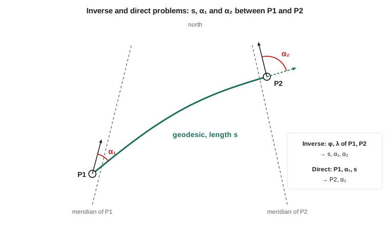
The 38 km pipeline that Coulee Geomatics is surveying for a gas utility runs north-east from a launcher site near Lethbridge, P1, to a receiver site, P2. The engineers need three numbers before they can lay out block valves and order pipe: the length of the line between the two sites on the ellipsoid, the azimuth in which to start at P1, and the azimuth at P2. Later, they will need the coordinates of points at given distances along the line. These are the two fundamental problems of geodetic computation. In the inverse problem, the coordinates of two points are known and the distance and azimuths between them are sought. In the direct problem, a starting point, an azimuth and a distance are known and the end point is sought. This lesson explains how both are solved on the ellipsoid, and why a sphere is not good enough.

Which line?

On a sphere, the shortest path between two points is an arc of a great circle, and the plane containing it passes through the centre. On an ellipsoid there are several candidate lines, and they are not the same. A normal section from A to B is the curve cut from the ellipsoid by the plane that contains the normal at A and the point B. It is what a theodolite set up and levelled at A sees when it sights B, apart from the deflection of the vertical. The normal section from B to A, containing the normal at B, is a different curve, because the two normals are skew lines that do not intersect in general. The two reciprocal normal sections enclose a thin sliver, and on a triangle of normal sections the angles do not close properly.

The geodesic is the unique shortest path on the surface between the two points. It lies between the two normal sections, roughly a third of the way from one to the other, and twists slightly. For lines of tens of kilometres the separation between the geodesic and either normal section is far below a millimetre and the lengths agree to better than a micrometre, so in practice the difference shows up only in angles, where it reaches a fraction of a second over a few hundred kilometres. Modern computation uses the geodesic because it is unique and has elegant properties. The most important is Clairaut's relation, which holds all along any geodesic:

Here \(N\cos\varphi\) is the radius of the parallel and \(\beta\) the reduced latitude. Clairaut's relation is the ellipsoidal counterpart of the fact that a great circle crosses each meridian at a predictable angle, and it makes the problem solvable.

Azimuths change along the line

Even a straight line on the ground does not keep a constant azimuth, because meridians converge toward the pole. On a line heading north-east, each successive meridian crossed is turned slightly clockwise relative to the last, so the azimuth grows. The difference between the forward azimuth at one end and the reverse of the back azimuth at the other is the convergence of meridians along the line. A good approximation is

where \(\varphi_m\) is the mean latitude. At the pipeline's latitude this is about 0.76 times the difference in longitude, close to 1100 arcseconds, or about 18 minutes, over 38 km. A surveyor who carried a constant bearing along the route would end up hundreds of metres off line. The same effect is why the reverse azimuth of a long line is not simply the forward azimuth plus 180°.

Methods of solution

Many methods have been devised. For lines up to a few tens of kilometres, series formulas such as the mid-latitude (Gauss) formulas are accurate to a few parts per million and can be evaluated by hand. They treat the line as if it lay on a sphere with radius of curvature \(M\) north–south and \(N\cos\varphi\) east–west at the mean latitude:

For longer lines, iterative methods are used. Thaddeus Vincenty published his formulas in 1975 for computers with little memory. They work on the auxiliary sphere of reduced latitudes, iterate on the difference in longitude, and are accurate to a fraction of a millimetre for any line that does not run between nearly antipodal points, where the iteration may fail to converge. Charles Karney's algorithms of 2013 solve the problem for all pairs of points, including antipodal ones, with errors of about 15 nanometres, and are now used in widely distributed geodetic software libraries. For the distances in this course, Vincenty's formulas and Karney's agree to well below a millimetre.

How Vincenty's inverse works

Vincenty's method maps each point to the auxiliary sphere using its reduced latitude, \(\tan\beta = (1-f)\tan\varphi\). On that sphere the geodesic becomes a great circle, but the longitude difference on the sphere, \(\lambda\), is not the same as the ellipsoidal one, \(L\). The algorithm starts with \(\lambda = L\), computes the angular distance \(\sigma\) on the sphere and the azimuth of the geodesic at the equator, and then applies a correction that makes \(\lambda\) slightly larger than \(L\). It repeats until \(\lambda\) stops changing, usually after three or four passes. Finally, it converts \(\sigma\) back to a length on the ellipsoid with a series in \(u^2 = e'^2\cos^2\alpha_0\), where \(\alpha_0\) is the azimuth at the equator, and computes the two azimuths from spherical trigonometry. The direct problem reverses these steps, iterating on \(\sigma\) instead.

The program below implements both directions in pure Python. As a check it first solves a published test line in Australia, from Flinders Peak to Buninyong, whose length on GRS80 is 54,972.271 m.

# Direct and inverse geodesic problems on GRS80 (Vincenty's formulae, pure Python)
import math

a, f = 6378137.0, 1 / 298.257222101
b = a * (1 - f)

def dms(d, m, s): return math.copysign(abs(d) + m / 60 + s / 3600, d)
def to_dms(x):
    sgn = "-" if x < 0 else ""; x = abs(x)
    d = int(x); m = int((x - d) * 60); s = (x - d - m / 60) * 3600
    return sgn + str(d) + " " + str(m).zfill(2) + " " + format(s, "08.5f")

def inverse(lat1, lon1, lat2, lon2):
    U1 = math.atan((1 - f) * math.tan(math.radians(lat1)))
    U2 = math.atan((1 - f) * math.tan(math.radians(lat2)))
    L = math.radians(lon2 - lon1); lam = L
    for it in range(200):
        sl, cl = math.sin(lam), math.cos(lam)
        ss = math.hypot(math.cos(U2) * sl, math.cos(U1) * math.sin(U2) - math.sin(U1) * math.cos(U2) * cl)
        cs = math.sin(U1) * math.sin(U2) + math.cos(U1) * math.cos(U2) * cl
        sig = math.atan2(ss, cs)
        sa = math.cos(U1) * math.cos(U2) * sl / ss
        c2a = 1 - sa * sa
        c2sm = cs - 2 * math.sin(U1) * math.sin(U2) / c2a
        C = f / 16 * c2a * (4 + f * (4 - 3 * c2a))
        prev = lam
        lam = L + (1 - C) * f * sa * (sig + C * ss * (c2sm + C * cs * (-1 + 2 * c2sm ** 2)))
        if abs(lam - prev) < 1e-12:
            break
    u2 = c2a * (a * a - b * b) / (b * b)
    A = 1 + u2 / 16384 * (4096 + u2 * (-768 + u2 * (320 - 175 * u2)))
    B = u2 / 1024 * (256 + u2 * (-128 + u2 * (74 - 47 * u2)))
    ds = B * ss * (c2sm + B / 4 * (cs * (-1 + 2 * c2sm ** 2) - B / 6 * c2sm * (-3 + 4 * ss ** 2) * (-3 + 4 * c2sm ** 2)))
    s = b * A * (sig - ds)
    az1 = math.degrees(math.atan2(math.cos(U2) * math.sin(lam), math.cos(U1) * math.sin(U2) - math.sin(U1) * math.cos(U2) * math.cos(lam))) % 360
    az2 = math.degrees(math.atan2(math.cos(U1) * math.sin(lam), -math.sin(U1) * math.cos(U2) + math.cos(U1) * math.sin(U2) * math.cos(lam))) % 360
    return s, az1, az2, it + 1          # az2 is the forward azimuth at point 2

def direct(lat1, lon1, az1, s):
    t = math.radians(az1)
    U1 = math.atan((1 - f) * math.tan(math.radians(lat1)))
    s1 = math.atan2(math.tan(U1), math.cos(t))
    sa = math.cos(U1) * math.sin(t); c2a = 1 - sa * sa
    u2 = c2a * (a * a - b * b) / (b * b)
    A = 1 + u2 / 16384 * (4096 + u2 * (-768 + u2 * (320 - 175 * u2)))
    B = u2 / 1024 * (256 + u2 * (-128 + u2 * (74 - 47 * u2)))
    sig = s / (b * A)
    for it in range(200):
        c2sm = math.cos(2 * s1 + sig)
        ds = B * math.sin(sig) * (c2sm + B / 4 * (math.cos(sig) * (-1 + 2 * c2sm ** 2) - B / 6 * c2sm * (-3 + 4 * math.sin(sig) ** 2) * (-3 + 4 * c2sm ** 2)))
        prev = sig; sig = s / (b * A) + ds
        if abs(sig - prev) < 1e-13:
            break
    c2sm = math.cos(2 * s1 + sig)
    num = math.sin(U1) * math.cos(sig) + math.cos(U1) * math.sin(sig) * math.cos(t)
    den = (1 - f) * math.hypot(sa, math.sin(U1) * math.sin(sig) - math.cos(U1) * math.cos(sig) * math.cos(t))
    lat2 = math.degrees(math.atan2(num, den))
    lam = math.atan2(math.sin(sig) * math.sin(t), math.cos(U1) * math.cos(sig) - math.sin(U1) * math.sin(sig) * math.cos(t))
    C = f / 16 * c2a * (4 + f * (4 - 3 * c2a))
    L = lam - (1 - C) * f * sa * (sig + C * math.sin(sig) * (c2sm + C * math.cos(sig) * (-1 + 2 * c2sm ** 2)))
    az2 = math.degrees(math.atan2(sa, -math.sin(U1) * math.sin(sig) + math.cos(U1) * math.cos(sig) * math.cos(t))) % 360
    return lat2, lon1 + math.degrees(L), az2

# Check against the published test line Flinders Peak -> Buninyong (Australia, GRS80)
s, a1, a2, n = inverse(-dms(37, 57, 3.72030), dms(144, 25, 29.52440), -dms(37, 39, 10.15610), dms(143, 55, 35.38390))
print("test line: s =", format(s, ".3f"), "m, az1 =", to_dms(a1), " reverse az =", to_dms((a2 + 180) % 360))

# Pipeline: launcher P1 to receiver P2
P1 = (dms(49, 41, 48.0), -dms(112, 49, 38.0))
P2 = (dms(49, 54, 50.0), -dms(112, 25, 10.0))
s, a1, a2, n = inverse(*P1, *P2)
print()
print("P1 -> P2 geodesic:", format(s, ",.3f"), "m in", n, "iterations")
print("  forward azimuth at P1", to_dms(a1), "; back azimuth at P2", to_dms((a2 + 180) % 360))
print("  azimuths differ by", round((a2 - a1) * 3600, 1), "arcsec (meridian convergence)")

lat2, lon2, az2 = direct(*P1, a1, s)                       # the direct problem returns P2
err = math.hypot((lat2 - P2[0]) * 3600 * 30.9, (lon2 - P2[1]) * 3600 * 20.0)   # about 30.9 m and 20.0 m per arcsec here
print("direct check: P2 recovered to", format(err * 1000, ".4f"), "mm")

R = 6371008.8                                               # sphere of mean radius
p1, p2, dl = math.radians(P1[0]), math.radians(P2[0]), math.radians(P2[1] - P1[1])
sph = R * math.acos(math.sin(p1) * math.sin(p2) + math.cos(p1) * math.cos(p2) * math.cos(dl))
print("sphere of mean radius gives", format(sph, ",.3f"), "m, a difference of", round(sph - s, 3), "m")

for km in (5, 10, 20, 30):                                  # block valve sites along the line
    la, lo, az = direct(*P1, a1, km * 1000.0)
    print("  station", str(km).rjust(3), "km:", to_dms(la), to_dms(lo), " azimuth there", round(az, 4))

test line: s = 54972.271 m, az1 = 306 52 05.37313  reverse az = 127 10 25.07026

P1 -> P2 geodesic: 38,018.100 m in 4 iterations
  forward azimuth at P1 50 23 14.02450 ; back azimuth at P2 230 41 55.36834
  azimuths differ by 1121.3 arcsec (meridian convergence)
direct check: P2 recovered to 0.0001 mm
sphere of mean radius gives 37,944.377 m, a difference of -73.723 m
  station   5 km: 49 43 31.14181 -112 46 25.68342  azimuth there 50.428
  station  10 km: 49 45 14.19432 -112 43 13.14045  azimuth there 50.4688
  station  20 km: 49 48 40.03065 -112 36 47.37412  azimuth there 50.5506
  station  30 km: 49 52 05.50743 -112 30 20.69863  azimuth there 50.6327

The test line reproduces the published length to the millimetre and the azimuths to a thousandth of a second, which gives confidence in the implementation. For the pipeline, the geodesic is 38,018.100 m long, starting at an azimuth of 50° 23′ 14.02″ and arriving at P2 heading 50° 41′ 55.37″, so the back azimuth from P2 is 230° 41′ 55.37″. The azimuths differ by 1121.3″, matching the convergence estimate. Feeding P1, the start azimuth and the length into the direct solution recovers P2 to a ten-thousandth of a millimetre. A sphere of mean radius gives a length 74 m short, an error of 0.19 per cent that no engineer would accept. The block valve coordinates, computed with the direct solution, show the azimuth creeping up by about 0.008° per kilometre.

Ellipsoid, grid and ground

The geodesic length is a distance on the ellipsoid, at zero ellipsoidal height. It is not the distance a total station measures on the ground, and it is not the distance between projected grid coordinates. A horizontal ground distance at height \(h\) is longer than the ellipsoidal distance by the factor \((R + h)/R\), about 140 parts per million at 900 m. A grid distance on a map projection differs from the ellipsoidal distance by the projection scale factor, which can be several hundred parts per million. Pipeline quantities are ordered from ground lengths, while legal descriptions and GIS databases often use grid values. Mixing them is a frequent cause of disputes. The reductions between the three are treated in GEOM-340; the geodesic computed here is the common reference from which both are derived.

Elevation along the route also matters. The pipeline follows the terrain, so its actual length includes the slope. Over gently rolling prairie the slope correction is small, but in coulees and river crossings it can add metres. The geodesic gives the horizontal component, and the profile adds the vertical one.

Where the computations are used

Inverse and direct computations appear everywhere in geodetic practice: in checking GNSS baselines against published coordinates, in computing the lengths and bearings of boundaries described by coordinates, in setting out long linear works, in maritime and aviation navigation, and in the reduction of observations in network adjustments. Geodetic software libraries provide them, but a surveyor should be able to recognize when results are wrong. The rough checks are simple: one arcsecond of latitude is about 31 m, one of longitude is about 31 cos φ m, azimuths of a north-easterly line increase along it by about \(\Delta\lambda\sin\varphi\), and the mid-latitude formulas agree with the rigorous answer to a few parts per million over tens of kilometres.