Geodetic networks

The pipeline's GNSS control was first established in 2012, adjusted to NAD83(CSRS) v6 from the stations then available. Now the utility wants the whole network in NAD83(CSRS) v8, and Coulee Geomatics has new observations tied to the Canadian Active Control System. Comparing old and new coordinates of the same marks shows differences of a few centimetres that are neither blunders nor monument movement: they come from a change of frame realization and from the motion of the crust between epochs. Handling this properly needs the ideas of the whole course: ellipsoid, ECEF coordinates, heights, rotation and time, all tied together in a reference frame realized by a network of stations. This final lesson describes how frames are defined and realized, how North American frames relate to the global ITRF, and how the seven-parameter transformation moves coordinates between frames.

Systems, frames and datums

Geodesists distinguish between a reference system and a reference frame. A reference system is a set of definitions: where the origin is, how the axes are oriented, what the unit of length is, how these evolve in time, and which ellipsoid and constants are used. A reference frame is the realization of a system: a catalogue of coordinates, and usually velocities, of physical stations, determined from observations. The word datum is used loosely for both, especially in older literature. The International Terrestrial Reference System (ITRS) is the ideal; ITRF2020 is its latest realization. NAD83 is a system; NAD83(CSRS) v8 and NAD83(2011) are realizations of it.

Because frames are realizations, they improve and change. Each new ITRF is computed from more years of data and better models, and its coordinates for the same station differ slightly from the previous version. A coordinate must therefore be labelled with the frame and its version. Because the stations move, it must also be labelled with the epoch, the instant to which it refers.

ITRF2020

ITRF2020, released in 2022 by the IERS, combines four space techniques, each contributing what it does best. Satellite laser ranging, which senses the Earth's centre of mass through satellite orbits, defines the origin. VLBI and satellite laser ranging together define the scale. The orientation follows a no-net-rotation condition, so that the frame does not rotate relative to the average motion of the plates. GNSS, with hundreds of globally distributed stations, densifies the frame and ties the techniques together at co-located sites, and DORIS adds a well-distributed network of beacons. ITRF2020 gives positions at a reference epoch of 2015.0, linear velocities, models of post-seismic deformation after large earthquakes and, for the first time, annual and semi-annual seasonal signals.

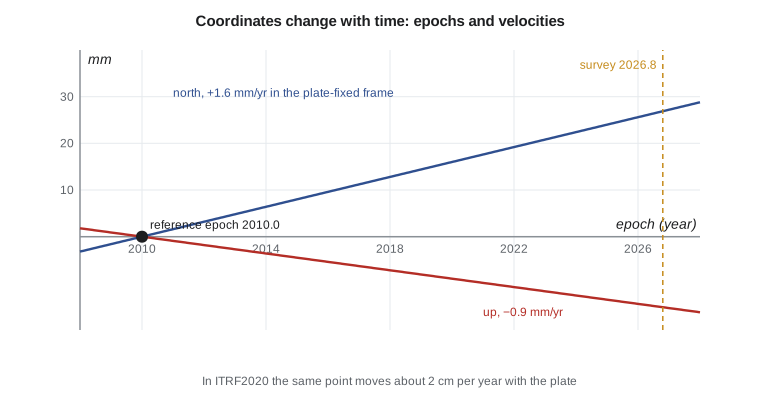
In ITRF2020, a station in southern Alberta or Montana moves by about 2 cm per year, mostly toward the south-west, as the North American plate rotates. Over a decade that is 20 cm, far too much to ignore. Global users accept this and work at the epoch of observation. National users usually prefer coordinates that stay fixed on a stable plate, so they adopt plate-fixed frames.

North American frames

NAD83 was defined in 1986 to be geocentric as well as the techniques of the day allowed, but its origin is now known to be about 2 m from the Earth's centre of mass, and its axes rotate with the North American plate. As a result, NAD83 and ITRF coordinates of the same point differ by one to two metres, and the difference changes by about 2 cm per year. NAD83(CSRS), the Canadian Spatial Reference System realization, has been issued in versions that track successive ITRFs: v5 based on ITRF2005 (epoch 2006.0), v6 on ITRF2008, v7 on ITRF2014 and v8, adopted in 2024, on ITRF2020, the last three at epoch 2010.0. Each version is defined by an exact transformation from the corresponding ITRF, published by Natural Resources Canada, and by a velocity model that moves coordinates between epochs.

The frame is realized in practice by active and passive control. The Canadian Active Control System of continuously operating GNSS stations, run by Natural Resources Canada, forms the primary framework, together with the Canadian Base Network of high-stability pillars. Provincial networks, such as Alberta's survey control markers and active networks, densify it. Users connect to the frame by processing against these stations or by precise point positioning with orbits and clocks consistent with the frame.

The seven-parameter transformation

When two frames are realizations of nearly the same system, the relation between them is close to a similarity transformation: a translation, a small rotation and a small change of scale. For ECEF coordinates,

with three translations \(\mathbf{T} = (t_x, t_y, t_z)\), a scale difference \(s\), usually given in parts per billion, and three rotations \(r_x\), \(r_y\), \(r_z\), usually given in milliarcseconds and small enough that their sines equal the angles and their products are negligible. This is the Helmert or Bursa–Wolf transformation. Its rotation matrix appears with two opposite sign conventions in the literature: the coordinate frame convention used here, in which the axes rotate, and the position vector convention, in which the point rotates. Using parameters from one convention in software that expects the other doubles the error instead of removing it, and on a regional scale a rotation of 20 mas is about 0.6 m. Always check the convention, ideally by transforming a published test point.

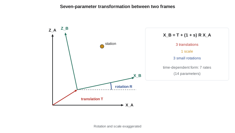
Frames whose stations move need time-dependent transformations. Each of the seven parameters is given as a value at a reference epoch plus a rate, making fourteen parameters, and coordinates must be propagated to a common epoch with velocities before or after the transformation. The ITRF2020 to NAD83 transformations of both countries take this form, and the plate rotation dominates their rates.

Estimating the parameters

When no published transformation exists, for example between an old local adjustment and a modern frame, the parameters are estimated by least squares from stations with coordinates in both. Each common station gives three observation equations, linear in the seven parameters, so at least three stations are needed and many more are desirable. The residuals show how well a similarity transformation fits; large residuals at one station suggest a disturbed mark or a blunder, and systematic patterns show distortions that seven parameters cannot absorb.

A regional network brings a particular difficulty. Over a small area, a rotation about an axis in the equatorial plane moves all points almost in parallel, just as a translation does, so the two are strongly correlated and individually poorly determined. The transformation of points inside the area can still be excellent, because the errors in the correlated parameters cancel. The program below demonstrates this with simulated data.

def T(A): return [list(r) for r in zip(*A)]
def mul(A, B): return [[sum(a * b for a, b in zip(r, c)) for c in zip(*B)] for r in A]
def inv(A):
    n = len(A); M = [list(map(float, r)) + [1.0 if i == j else 0.0 for j in range(n)] for i, r in enumerate(A)]
    for c in range(n):
        p = max(range(c, n), key=lambda r: abs(M[r][c])); M[c], M[p] = M[p], M[c]
        d = M[c][c]; M[c] = [x / d for x in M[c]]
        for r in range(n):
            if r != c:
                f = M[r][c]; M[r] = [x - f * y for x, y in zip(M[r], M[c])]
    return [r[n:] for r in M]
def diag(v): return [[v[i] if i == j else 0.0 for j in range(len(v))] for i in range(len(v))]
def col(v): return [[x] for x in v]
# Seven-parameter (Helmert) transformation estimated by least squares from common stations
import math, random

a, f = 6378137.0, 1 / 298.257222101
e2 = f * (2 - f)
def ecef(lat, lon, h):
    p, l = math.radians(lat), math.radians(lon)
    N = a / math.sqrt(1 - e2 * math.sin(p) ** 2)
    return [(N + h) * math.cos(p) * math.cos(l), (N + h) * math.cos(p) * math.sin(l), (N * (1 - e2) + h) * math.sin(p)]

MAS = math.radians(1 / 3600 / 1000)          # one milliarcsecond in radians
def helmert(X, p):                            # p = tx, ty, tz (m), s (ppb), rx, ry, rz (mas); small angles
    tx, ty, tz, s, rx, ry, rz = p
    k = 1 + s * 1e-9; rx, ry, rz = rx * MAS, ry * MAS, rz * MAS
    x, y, z = X
    return [tx + k * (x + rz * y - ry * z), ty + k * (-rz * x + y + rx * z), tz + k * (ry * x - rx * y + z)]

# Common stations: coordinates in the old adjustment (frame A) across a regional network
sites = [(49.70, -112.83, 900), (51.08, -114.13, 1100), (53.55, -113.50, 700), (50.45, -104.61, 580),
         (52.13, -106.67, 500), (49.27, -123.12, 60), (48.42, -114.34, 950), (55.17, -118.80, 650)]
A = [ecef(*s) for s in sites]
TRUE = [0.912, -1.304, -0.481, 12.0, 26.0, -14.0, 19.0]    # parameters used to simulate frame B
rnd = random.Random(230)
B = [[c + rnd.gauss(0, 0.004) for c in helmert(X, TRUE)] for X in A]   # 4 mm noise per coordinate

# Linearized model: B - A = J p, with columns for tx, ty, tz, s, rx, ry, rz
Jrows, d = [], []
for X, Y in zip(A, B):
    x, y, z = X
    Jrows += [[1, 0, 0, x * 1e-9, 0, -z * MAS, y * MAS],
              [0, 1, 0, y * 1e-9, z * MAS, 0, -x * MAS],
              [0, 0, 1, z * 1e-9, -y * MAS, x * MAS, 0]]
    d += [Y[0] - x, Y[1] - y, Y[2] - z]
Nm = mul(T(Jrows), Jrows); Qx = inv(Nm)
p = [r[0] for r in mul(Qx, mul(T(Jrows), col(d)))]
v = [sum(J * q for J, q in zip(row, p)) - di for row, di in zip(Jrows, d)]
dof = len(d) - 7
s0 = math.sqrt(sum(x * x for x in v) / dof)
names = ["tx (m)", "ty (m)", "tz (m)", "scale (ppb)", "rx (mas)", "ry (mas)", "rz (mas)"]
print("parameter       estimate     sigma      simulated")
for i, n in enumerate(names):
    print(n.ljust(12), format(p[i], "10.4f"), format(s0 * math.sqrt(Qx[i][i]), "10.4f"), format(TRUE[i], "10.4f"))
print("residual standard deviation =", round(1000 * s0, 1), "mm with", dof, "degrees of freedom")
corr = Qx[0][5] / math.sqrt(Qx[0][0] * Qx[5][5])
print("correlation between tx and ry =", round(corr, 3))

# Apply the estimated parameters to a pipeline point
P = ecef(49.9139, -112.4194, 905.0)
Q = helmert(P, p)
print("pipeline P2 shifts by dX, dY, dZ =", [round(q - c, 4) for q, c in zip(Q, P)], "m")
x, y, z = P
JP = [[1, 0, 0, x * 1e-9, 0, -z * MAS, y * MAS], [0, 1, 0, y * 1e-9, z * MAS, 0, -x * MAS], [0, 0, 1, z * 1e-9, -y * MAS, x * MAS, 0]]
CP = mul(mul(JP, Qx), T(JP))
print("standard deviation of the transformed P2 =", [round(1000 * s0 * math.sqrt(CP[i][i]), 1) for i in range(3)], "mm")

# Same data, translations only: what the three-parameter model leaves behind
t = [sum(d[i::3]) / len(A) for i in range(3)]
v3 = [d[i] - t[i % 3] for i in range(len(d))]
print("three-parameter fit residual RMS =", round(1000 * math.sqrt(sum(x * x for x in v3) / (len(d) - 3)), 1), "mm")

parameter       estimate     sigma      simulated
tx (m)           0.9284     0.0248     0.9120
ty (m)          -1.2909     0.0312    -1.3040
tz (m)          -0.4487     0.0286    -0.4810
scale (ppb)     10.5120     3.1197    12.0000
rx (mas)        24.9441     1.1787    26.0000
ry (mas)       -13.4718     0.8197   -14.0000
rz (mas)        19.3994     0.6874    19.0000
residual standard deviation = 4.0 mm with 17 degrees of freedom
correlation between tx and ry = 0.848
pipeline P2 shifts by dX, dY, dZ = [0.8713, -0.5958, 0.1649] m
standard deviation of the transformed P2 = [1.5, 1.6, 1.7] mm
three-parameter fit residual RMS = 32.6 mm

Eight stations spread across the prairies and mountains were transformed with the simulated parameters and given 4 mm of random noise. The least-squares solution recovers the residual standard deviation of 4.0 mm, and every parameter lies within about two standard deviations of its simulated value. The translations are uncertain by 2 to 3 cm and the scale by about 3 ppb, and the correlation between \(t_x\) and \(r_y\) is 0.85. Yet the transformed coordinates of the pipeline's P2 are uncertain by only 1.5 to 1.7 mm, because P2 lies inside the network where the correlated errors cancel. A translation-only fit leaves residuals of 33 mm, showing that the rotations and scale are needed. The lesson for practice: judge a transformation by its residuals and by the precision of transformed points inside the area, not by the parameters themselves, and do not extrapolate it far outside the stations used.

Networks in practice

Geodetic networks today are hierarchical but far flatter than the triangulation chains of the past. At the top are the global frame and the continuously operating stations that realize the national frame. Below them, high-accuracy passive marks and real-time networks bring the frame within reach of every project. Project control, such as the pipeline's GNSS network or the bridge's pillars, is tied to that framework and adjusted with its stations held fixed or weighted, as in GEOM-220. Accuracy standards express the result as network accuracy, relative to the frame, and local accuracy, relative to neighbouring points, both at 95 per cent confidence.

The ideas of this course come together in such a network. Positions are ECEF coordinates on GRS80, converted to latitude, longitude and ellipsoidal height. Heights become physical heights through a geoid model referred to a potential \(W_0\). Directions measured with levelled instruments must allow for the deflection of the vertical. The frame itself is tied to the stars and quasars through Earth rotation parameters, and it moves with the crust, so every coordinate carries an epoch. When frames change, the seven or fourteen parameter transformation carries old coordinates into the new frame. A surveyor who understands each step can explain to a client why the numbers changed, and can prove that the ground did not.