
ENGG-401 · Lesson 3 of 12 · 30 min
Equivalence factors: uniform series and gradients
Real projects rarely involve a single payment. Equipment saves money every year, loans are repaid monthly, maintenance costs rise as assets age, and energy prices grow over time. Rather than discounting every cash flow individually, engineering economics uses a set of standard factors that convert whole series of cash flows into equivalent present, future or annual amounts. This lesson derives and applies the uniform series factors, the arithmetic and geometric gradient factors, deferred series, perpetuities and capitalized cost, explains factor notation and tables, and shows how spreadsheets calculate the same results.
Factor notation
Each factor is written in the form \((X/Y, i, n)\), read as "find X given Y at interest rate i over n periods". For example, \((P/A, 8\,\%, 10)\) is the factor that converts a uniform annual amount \(A\) over 10 periods into its present worth \(P\) at 8 %. Multiplying the known amount by the factor gives the unknown: \(P = A\,(P/A, i, n)\). The notation makes equations easy to read and check: the units cancel like fractions, \(A \times P/A = P\). Interest tables at the back of engineering economics textbooks list the factors for common rates and periods; today they are usually calculated by spreadsheet or calculator, but the notation remains standard, including on the NCEES Fundamentals of Engineering exam and in Canadian engineering programs.
Uniform series factors
A uniform series consists of equal amounts \(A\) at the end of each period from 1 to \(n\). Summing the compound amounts of each payment gives the uniform series compound amount factor:
Its inverse, the sinking fund factor, gives the uniform amount that must be deposited each period to accumulate a future sum:
Combining with the single-payment factors gives the uniform series present worth factor, which converts a series into a present amount, and its inverse, the capital recovery factor, which converts a present amount into an equivalent uniform series, such as the annual payment on a loan:
A useful identity links them: \((A/P, i, n) = (A/F, i, n) + i\). The capital recovery factor equals the sinking fund factor plus the interest rate, because recovering capital means both earning interest on it and replacing it.
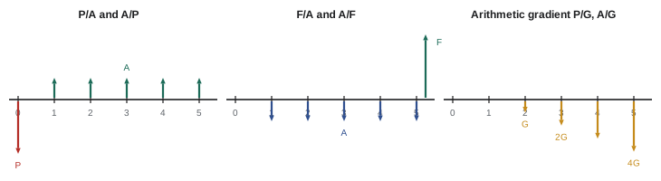
| Factor | i = 5 % | i = 8 % | i = 10 % |
|---|---|---|---|
| (F/P, i, 10) | 1.6289 | 2.1589 | 2.5937 |
| (P/F, i, 10) | 0.6139 | 0.4632 | 0.3855 |
| (F/A, i, 10) | 12.5779 | 14.4866 | 15.9374 |
| (A/F, i, 10) | 0.0795 | 0.0690 | 0.0627 |
| (P/A, i, 10) | 7.7217 | 6.7101 | 6.1446 |
| (A/P, i, 10) | 0.1295 | 0.1490 | 0.1627 |
| (P/G, i, 10) | 31.6520 | 25.9768 | 22.8913 |
| (A/G, i, 10) | 4.0991 | 3.8713 | 3.7255 |
Applying uniform series factors
Worked problem
Capital recovery for a loan
A municipality borrows $2,000,000 for a pumping station at 7 % per year, repaid in 20 equal annual payments. What is the annual payment?
Show solution
- Find \(A\) given \(P\): \(A = P\,(A/P, 7\,\%, 20)\).
- \((A/P, 7\,\%, 20) = \dfrac{0.07 \times 1.07^{20}}{1.07^{20} - 1} = 0.09439\).
- \(A = 2{,}000{,}000 \times 0.09439 = 188{,}786\).
Answer: About $188,786 per year for 20 years.
Worked problem
A sinking fund for replacement
A plant wants to accumulate $500,000 in 8 years to replace a boiler. The fund earns 5 % per year. How much must be deposited at the end of each year?
Show solution
- \(A = F\,(A/F, 5\,\%, 8) = 500{,}000 \times \dfrac{0.05}{1.05^{8} - 1}\).
- \(1.05^8 = 1.4775\), so the factor is \(0.05/0.4775 = 0.10472\).
- \(A = 500{,}000 \times 0.10472 = 52{,}361\).
Answer: About $52,361 per year.
Arithmetic gradients
Many costs increase by a roughly constant amount each year, such as maintenance on ageing equipment. An arithmetic gradient series has cash flows of \(0, G, 2G, \dots, (n-1)G\) at the ends of periods 1 to \(n\). By convention, the gradient begins at the end of period 2; a series that starts at a base amount \(A_1\) in period 1 and increases by \(G\) each period is treated as a uniform series of \(A_1\) plus a pure gradient. The gradient factors are:
Worked problem
Rising maintenance costs
Maintenance on a conveyor costs $2,000 in year 1 and rises by $500 each year for 10 years. At 8 %, what is the present worth of maintenance, and the equivalent uniform annual cost?
Show solution
- Base series: \(2{,}000\,(P/A, 8\,\%, 10) = 2{,}000 \times 6.7101 = 13{,}420\).
- Gradient: \(500\,(P/G, 8\,\%, 10) = 500 \times 25.9768 = 12{,}988\).
- Present worth: \(13{,}420 + 12{,}988 = 26{,}409\).
- Equivalent annual cost: \(2{,}000 + 500\,(A/G, 8\,\%, 10) = 2{,}000 + 500 \times 3.8713 = 3{,}936\).
Answer: Present worth about $26,409; equivalent uniform annual cost about $3,936.
Geometric gradients
Some cash flows grow by a constant percentage rather than a constant amount: energy costs rising with inflation, revenues growing with market share, wages rising each year. A geometric gradient series starts at \(A_1\) in period 1 and grows at rate \(g\) per period, so the cash flow in period \(t\) is \(A_1(1 + g)^{t-1}\). Its present worth is:
Worked problem
Escalating energy costs
A motor upgrade saves 400,000 kWh per year. Electricity costs $0.10 per kWh in year 1 and is expected to rise 3 % per year. Over 15 years at a MARR of 9 %, what is the present worth of the savings?
Show solution
- Year 1 savings: \(A_1 = 400{,}000 \times 0.10 = 40{,}000\).
- Factor: \(\dfrac{1 - (1.03/1.09)^{15}}{0.09 - 0.03} = \dfrac{1 - 0.4277}{0.06} = 9.538\).
- Present worth: \(40{,}000 \times 9.538 = 381{,}520\).
- Without escalation, \(40{,}000\,(P/A, 9\,\%, 15) = 40{,}000 \times 8.0607 = 322{,}428\), so escalation adds about 18 %.
Answer: About $381,500; ignoring escalation would undervalue the savings by about $59,000.
Deferred series and shifted cash flows
Series that do not start at period 1 are handled in two steps: find the equivalent value one period before the series begins using the series factor, then discount that value to time 0. For a uniform series from year 4 to year 10, the \((P/A)\) factor gives a value at year 3, which is then multiplied by \((P/F, i, 3)\). Errors in locating this intermediate point are among the most common in engineering economics; drawing the cash flow diagram and marking where each factor places its result avoids them.
At 8 %, a series of $10,000 a year from years 4 to 10 has \(P = 10{,}000 \times 5.2064 \times 0.7938 = 41{,}330\).
Perpetuities and capitalized cost
When a uniform series continues indefinitely, such as the maintenance of a permanent public work or an endowment, the present worth factor approaches \(1/i\) as \(n\) becomes large. The present worth of a perpetual annual amount is therefore \(P = A/i\). Capitalized cost is the present worth of an asset assumed to provide service forever, including its first cost and all future costs. For example, a dam with annual maintenance of $100,000 at a discount rate of 5 % has a capitalized maintenance cost of \(100{,}000/0.05 = 2{,}000{,}000\). Periodic costs that recur every \(k\) years, such as a major overhaul every 20 years, are first converted to an equivalent annual amount using \((A/F, i, k)\), then capitalized. Capitalized cost is used for infrastructure such as tunnels, dams, canals and endowed facilities, where very long lives make the infinite-horizon approximation reasonable.
Spreadsheet functions
Spreadsheets implement these factors as financial functions. In Excel, Google Sheets and similar programs, PV(rate, nper, pmt, fv) gives present value, FV gives future value, PMT gives the uniform payment, NPV discounts a range of cash flows starting at period 1 (so the time 0 cash flow must be added separately), RATE and IRR find interest rates, and NPER finds the number of periods. These functions follow a cash flow sign convention in which money paid out is negative, so results often appear with a negative sign. Spreadsheets are essential for irregular cash flows and for sensitivity analysis, but understanding the factors remains important for setting up problems correctly, checking results and working without software, as in licensing exams.
| Task | Factor | Spreadsheet function |
|---|---|---|
| Present worth of a uniform series | (P/A, i, n) | =PV(i, n, −A) |
| Future worth of a uniform series | (F/A, i, n) | =FV(i, n, −A) |
| Loan payment | (A/P, i, n) | =PMT(i, n, −P) |
| Sinking fund deposit | (A/F, i, n) | =PMT(i, n, 0, −F) |
| Present worth of irregular flows | Sum of (P/F) terms | =NPV(i, flows 1..n) + flow 0 |
Shifted gradients and combined patterns
Real cash flow patterns often combine several elements: a first cost, a uniform series of revenues starting after a construction period, a gradient of rising maintenance, and periodic overhauls. The reliable method is to break the pattern into standard pieces, value each piece with the appropriate factor at the point where that factor places its result, discount each result to time 0, and add. For example, a plant that takes two years to build, then earns revenues that grow by a constant amount each year, has a gradient series whose P/G value lands at the end of year 2, one period before the first revenue; it is then discounted two years. Decreasing gradients, such as revenues that fall as equipment ages, are handled by subtracting a gradient from a uniform series. Writing each piece clearly, with its factor and location, makes complex problems manageable and easy to check.
Interpolating in interest tables
When tables are used and the needed interest rate or number of periods is not listed, linear interpolation between neighbouring entries gives a close approximation. For example, \\((P/A, 7.5\\,\\%, 10)\\) lies between \\((P/A, 7\\,\\%, 10) = 7.0236\\) and \\((P/A, 8\\,\\%, 10) = 6.7101\\), and interpolation gives about 6.8669, very close to the exact value of 6.8641. Interpolation is less accurate over wide intervals because factors are non-linear functions of the interest rate, and calculating factors directly from their formulas or with a spreadsheet avoids the issue entirely.
Checking factor calculations
Because factor errors are easy to make, simple checks are valuable. The present worth of a uniform series must be less than the undiscounted sum \\(nA\\) and greater than \\(A\\); at \\(i = 0\\), \\((P/A, 0, n) = n\\). The future worth of a uniform series must exceed \\(nA\\). The capital recovery factor must exceed \\(1/n\\), because it includes interest, and approaches \\(i\\) as \\(n\\) grows large. Gradient present worths should be checked against a rough sum of discounted values for a few years. Finally, for any complex problem, a spreadsheet that discounts each cash flow individually provides an independent check of factor-based calculations. Developing the habit of estimating whether an answer is reasonable before trusting it prevents many errors, in coursework and in professional practice.
Factors with continuous compounding
With continuous compounding at nominal rate \\(r\\), the single-payment factors become \\(e^{rn}\\) and \\(e^{-rn}\\), and the uniform series present worth factor becomes \\((e^{rn} - 1)/(e^{rn}(e^{r} - 1))\\). For cash flows that occur continuously and uniformly through each period, such as energy savings, the funds-flow present worth factor is \\((e^{rn} - 1)/(r\\,e^{rn})\\). These forms appear in some textbooks and in the FE exam reference handbook, and give results slightly different from end-of-period discrete compounding, typically by a few per cent.
Factor notation also makes problems easier to communicate: a reviewer reading P = 15,000 (P/A, 8 %, 10) knows exactly what was assumed, which is why professional reports and licensing exams continue to use it even when spreadsheets do the arithmetic.
Common mistakes
MistakePlacing the result of a P/A factor at the start of the series.
InsteadP/A places the result one period before the first payment.
MistakeStarting an arithmetic gradient in period 1.
InsteadThe gradient starts in period 2; treat the base as a uniform series.
MistakeUsing the Excel NPV function on time 0 cash flows.
InsteadAdd the time 0 flow separately.
MistakeIgnoring escalation in long-lived savings.
InsteadUse geometric gradients where costs grow by a percentage.
MistakeTreating a perpetuity with a finite-life factor.
InsteadUse P = A/i for indefinite series.
Summary and key terms
- Factors in the form (X/Y, i, n) convert known amounts into equivalent unknowns.
- F/A and A/F relate uniform series to future amounts; P/A and A/P to present amounts.
- A/P equals A/F plus i.
- Arithmetic gradients increase by G each period starting in period 2.
- Geometric gradients grow by a percentage g each period.
- Deferred series are valued one period before they begin, then discounted.
- Perpetuities have P = A/i; capitalized cost values assets with indefinite lives.
- Uniform series
- Equal end-of-period amounts from period 1 to n.
- Capital recovery factor
- A/P, converting a present amount to an annual series.
- Sinking fund factor
- A/F, the deposit needed to reach a future sum.
- Uniform series present worth factor
- P/A, converting a series to present worth.
- Arithmetic gradient
- Cash flows increasing by a constant amount.
- Geometric gradient
- Cash flows growing by a constant percentage.
- Deferred series
- Series starting after period 1.
- Perpetuity
- Series continuing indefinitely.
- Capitalized cost
- Present worth of an asset with an indefinite life.
- Escalation
- Growth of costs over time.
Practice problems
Work each problem on paper first, then reveal the answer to check.
Present worth of $15,000 a year for 10 years at 8 %?
Show answer
About $100,651.
Future worth of $1,000 a year for 10 years at 5 %?
Show answer
About $12,578.
Annual payment on $100,000 at 10 % over 10 years?
Show answer
About $16,275.
What is A/P minus A/F?
Show answer
The interest rate i.
When does an arithmetic gradient begin?
Show answer
At the end of period 2.
Equivalent annual cost of a gradient of $1,000 over 10 years at 10 %?
Show answer
About $3,726.
Present worth of a perpetual $50,000 per year at 4 %?
Show answer
$1,250,000.
Where does P/A place the value of a series from years 6 to 15?
Show answer
At year 5.
Which formula applies when g = i in a geometric series?
Show answer
P = n A₁/(1 + i).
Why add time 0 separately with NPV in a spreadsheet?
Show answer
The function starts discounting at period 1.
Lesson quiz · 5 questions
Score 60% or more to complete this lesson.
Create a free account to save your progress, take quizzes and earn a certificate.